If you like this blog post, do subscribe to my RSS feed

GADDAG

The Secret World of Data Structures and Algorithms, Chapter 3

Author: Parth Parikh

First Published: 22/06/23

Words are, in my not-so-humble opinion, our most inexhaustible source of magic. Capable of both inflicting injury, and remedying it.
- Albus Dumbledore, from J.K. Rowling's Harry Potter and the Deathly Hallows

Welcome to the draft of the third chapter of my journey to write a short book on data structures and algorithms that are not widely known outside of academic circles. We have previously covered KHyperLogLog and Odd Sketches. As always, I'm looking forward to your feedback , which is greatly appreciated.

In this chapter, we will be discussing GADDAG, a data structure that efficiently generates moves in Scrabble.

Introduction

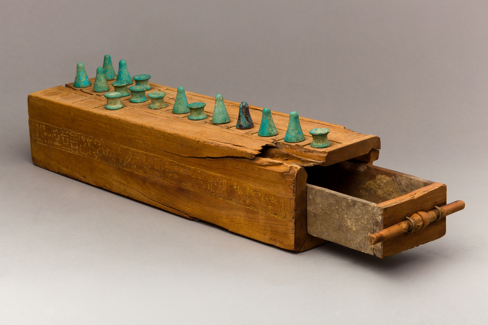
Throughout history, humans have always been captivated by board games. One of the earliest discovered games is the Egyptian board game, Senet, dating back to around 3500 BCE. The game featured a board of thirty squares, arranged into three parallel rows with ten squares each, with pieces (known as draughtsmen) being moved across the board. Although the exact rules of the game are still a mystery, it is believed that the objective was to reach the edge of the board first, and accomplishing this may have had some significance towards the afterlife. Pieces were moved based on the throw of sticks or bones. According to a 1980 article by Peter A. Piccione:

This research demonstrates that the stratagems of the game reflect nothing less than the stratagems of the gods, and that senet, when properly understood, can reveal essential Egyptian religious beliefs about the afterlife. At the most, the game indicates that ancient Egyptians believed they could join the god of the rising sun, Re-Horakhty, in a mystical union even before they died. At the least, senet shows that, while still living, Egyptians felt they could actively influence the inevitable afterlife judgment of their souls - a belief that was not widely recognized by Egyptologists.

Senet was originally strictly a pastime with no religious significance. As the Egyptian religion evolved and fascination with the netherworld increased - reflected in such ancient works as the Book of Gates, Book of What is in the Netherworld, and portions of the Book of the Dead - the Egyptians superimposed their beliefs onto the gameboard and specific moves of senet. By the end of the Eighteenth Dynasty in 1293 BC, the senet board had been transformed into a simulation of the netherworld, with its squares depicting major divinities and events in the afterlife.

Perhaps equally fascinating is our desire to become the absolute best at these board games. A remarkable example of this is the 1984 chess world championship between Garry Kasparov and Anatoly Karpov. Karpov was the reigning world champion going into the tournament and the rules stated that the first player to win six games would be crowned the champion (draws were not counted). The match was fiercely fought over five months, and a total of 48 games were played. However, neither player won the required six games to claim the title. It was eventually halted without a winner, with a follow-up scheduled five months later.

In recent history, our hunger to understand board games has prompted us to explore the use of computers to dominate them. This drive partly arises from our desire to uncover game secrets and expand our thinking into new dimensions. An intriguing anecdote, which is somewhat antithetical in this context, involves yet another chess world championship match between Garry Kasparov and Vladimir Kramnik in 2000. As chess engines gained in prominence, they began to reveal innovative lines employed by grandmasters, but there were still many openings that remained a mystery to these engines. One such enigma was the Berlin Defense, a variation of the centuries-old Ruy Lopez that had been largely forgotten. However, Kramnik utilized the defense to draw against Kasparov with the black pieces, as it was widely believed that computer engines struggled to understand this opening at the time. This technique propelled Kramnik to victory, as he went on to be crowned the new world champion. Later on, computer engines developed incredible defensive resources using the Berlin Defense, and it is now widely used among top-level chess players.

But in this chapter, we are not going to talk about Senet or Chess. Instead, we will discuss Scrabble. In particular, we will explore two fascinating data structures called DAWG and GADDAG that helped pave the way for computer domination in the world of Scrabble playing.

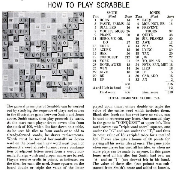
Alfred Butts, the creator of Scrabble, spent much of his later life in seclusion; however, his inspiration behind the game's creation was fascinatingly shared in a 1953 article in Life magazine:

Scrabble is not, in fact, new. It has been swimming around in the brain of a mild, bespectacled, New York architect named Alfred Butts for about 20 years. Early in the Depression, Butts found himself temporarily unemployed. Casting about for some means of making a living, he decided to invent a game. He disliked dice games, which are almost entirely luck, and felt that all-skill games, like chess, were too highbrow for the general market. A game which was half luck and half skill, he thought, would be about right. He had always enjoyed anagrams and crossword puzzles and so set out to combine these games within the luck-skill formula. After two or three years of experiment he developed the thing that is now Scrabble, although he never found a satisfactory name and referred to it simply as “it”.

Directed Acyclic Word Graphs

In 1988, Andrew Appel and Guy Jacobson presented an intriguing algorithm for rapidly generating Scrabble moves. But before we delve into the nitty-gritty of the algorithm, let's first take a step back and truly understand the problem we're attempting to solve here.

Specifically, our focus is on generating moves in Scrabble. This means that given a turn, we aim to identify viable moves that a player can make using the letters both on their rack and on the game board.

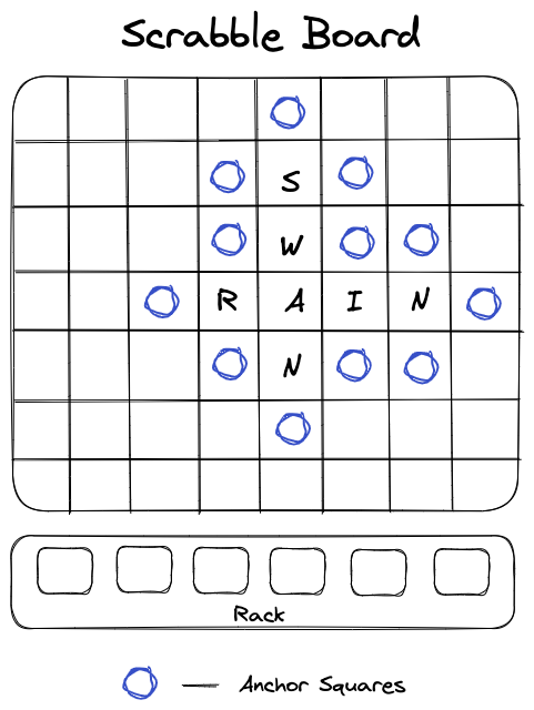
Throughout this chapter, we will be using the term anchor squares. An anchor square refers to any square on the board onto which letters can be hooked to create new words. It's easy to identify the anchor squares by finding the empty squares that are adjacent (vertically or horizontally) to filled squares. Figure 3 provides a visualization of this concept.

To determine possible valid moves, it is crucial to maintain a data structure that searches through parts of a lexicon in order to gather valid moves. But what would this data structure look like?

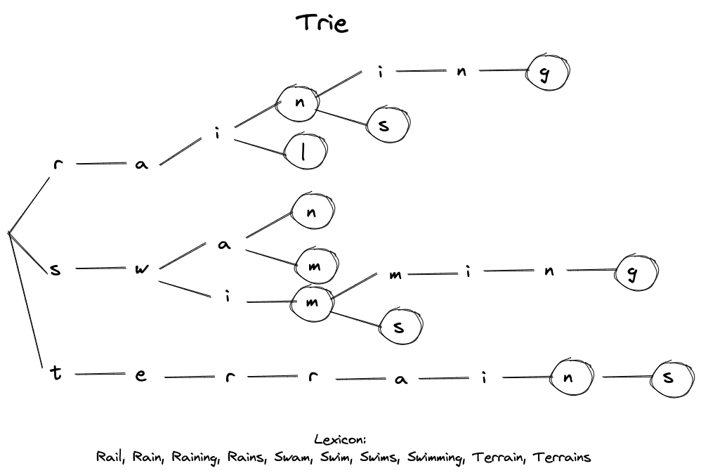
A potential solution would be to use a trie. A trie is a tree-like data structure that can be used to test whether a particular string is present in the set of strings. The root node represents an empty string, and each node represents a possible continuation of the string. For instance, a trie that represents the entire English lexicon would have 26 nodes (for the letters A to Z) as children to the root node, and it would further branch out from there. A visualization of a trie for a subset of the English lexicon is shown in the figure 4.

Tries are simple to build, as one can easily insert new strings repeatedly. They are also fast to search, but they consume a lot of space. This can be easily visualized by considering the number of repetitions that occur in a trie when words ending with -s, -ed, or -ing are encountered.

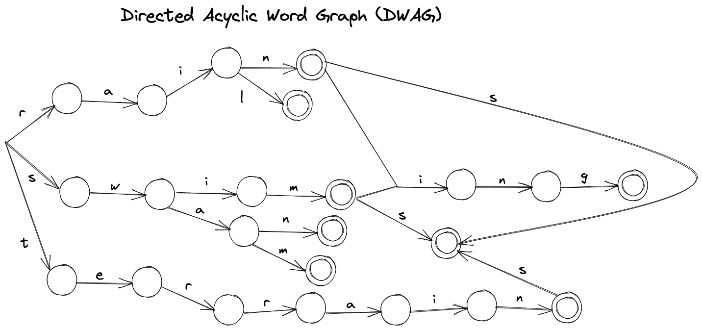
When Appel and Jacobson experimented with tries, they discovered that a 94,240-word lexicon could be represented by a 117,150-node trie with 179,618 edges. To improve this naive solution, they suggested using a Directed Acyclic Word Graph (DAWG). A DAWG is a finite state machine where the nodes represent its states, the edges show the transition, and the terminal nodes represent the accepted states - or in our case, the words within a lexicon. However, it's worth noting that there can be multiple finite state machines derived from a lexicon. Therefore, DAWG is the minimized finite state machine, ensuring that all equivalent sub-tries merge - for example, words that end with -s, -ed, or -ing. A visual depiction of this structure with the same lexicon is shown in the figure 5.

Using DAWG, Appel, and Jacobson reduced the 117,150-node trie to 19,853 nodes.

But how do we parse a DAWG? To begin, let's define the concept of a left part of a word. This refers to the segment of a word that starts from the left of the anchor square. It can include letters from either the rack or the board, but not both simultaneously. Similarly, a right part of a word consists of a segment including and to the right of the anchor square. With this in mind, we can use a two-part strategy:

1. Identify all possible left parts of a word anchored at a given anchor.
2. For each left part, find all suitable right parts.

The way vertical words are treated is by considering them as horizontal words with the board transposed.

Here is a recursive algorithm to compute the left parts.

LeftPart(\(PartialWord\), \(N\), \(Limit\)):
1. ExtendRight(\(PartialWord\), \(N\), \(AnchorSquare\))
2. If \(Limit > 0\):
1. For each edge \(E\) from \(N\):
1. If letter \(L\) on edge \(E\) is in rack:
1. Remove \(L\) from rack
2. LeftPart(\(PartialWord \cdot L\), node reached from \(E\), \(Limit - 1\))
3. Return \(L\) to rack

To generate all the moves from the \(AnchorSquare\), a LeftPart(" ", root node \(N\), \(Limit\)) call can be made, where \(Limit\) is the number of non-anchor squares to the left of the \(AnchorSquare\).

The right parts can then be computed as follows:

ExtendRight(\(PartialWord\), \(N\), \(Square\)):
1. If \(Square\) is vacant:
1. If \(N\) is terminal node:
1. LegalMove(\(PartialWord\))
2. For each edge \(E\) from \(N\):
1. If letter \(L\) on edge \(E\) is in rack:
1. Remove \(L\) from rack
2. ExtendRight(\(PartialWord \cdot L\), node reached from \(E\), square to the right of \(Square\))
3. Return \(L\) to rack
2. Else:
1. \(L =\) letter occupying \(Square\)
2. If node \(N\) has an out-edge \(L\):
1. ExtendRight(\(PartialWord \cdot L\), node reached from out-edge \(L\), square to the right of \(Square\))

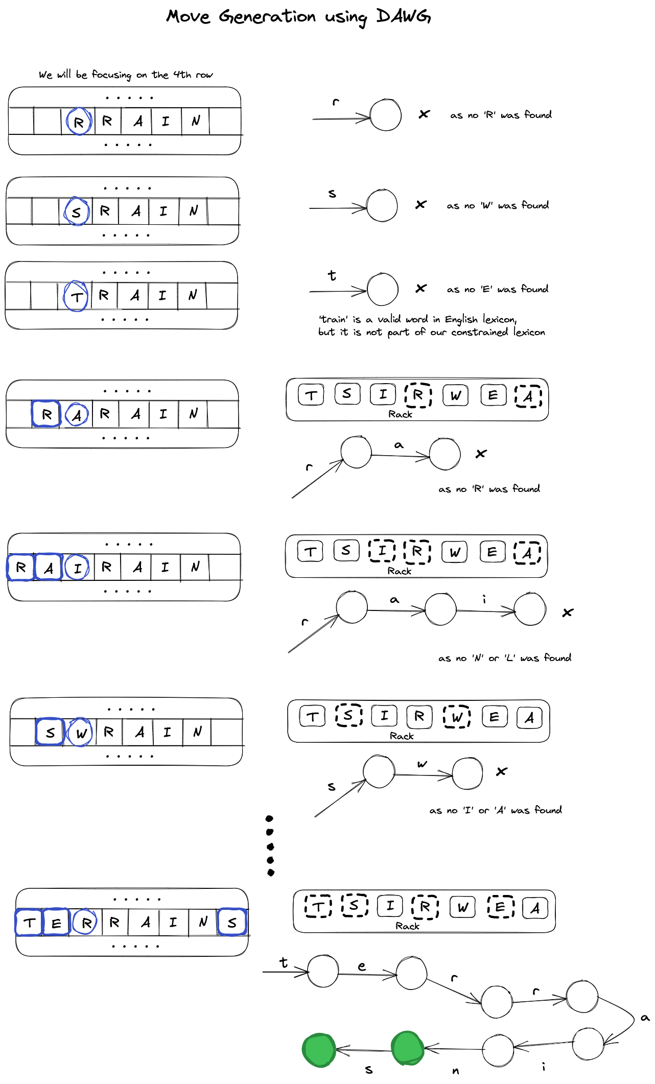
Here's a visual of parsing a DAWG from an \(AnchorSquare\). As you can see, in the case of two squares, we ultimately find two valid words: "terrain" and "terrains". "ter-" serves as the prefix and "-s" the suffix for the latter.

One of the major pain points of DAWG is the unconstrained generation of prefixes. As the words are only generated from left to right, the part that focuses on the calculation of prefixes is crucial. However, there may be scenarios where prefixes cannot be completed with any remaining tiles in the rack, or where prefixes cannot be completed using the letters on the board that the algorithm must go through. By using the above approach, we can see that a considerable amount of backtracking would be necessary for such situations.

So, how can we improve on this limitation? Approximately five years after DAWG, Steven Gordon published a paper introducing GADDAG, a data structure that avoids the non-deterministic prefix generation method used by DAWG. Gordon's approach creates bidirectional paths for every word starting at each letter. While Gordon's approach remains non-deterministic, it is more deterministic than Appel and Jacobson's approach. In the following section, we will explore this data structure.

GADDAG

The key idea in GADDAG that enables bidirectional paths is the fact that a language such as \[L = \{REV(x)\diamond y \;|\; xy \text{ is a word and } x \text{ is not empty}\}\] can be used to avoid non-deterministic prefix generation. Here, \(REV(x)\) is the reverse string of \(x\) and \(\diamond\) is a delimiter. So, what does this mean for the language \(L\) and how does it make GADDAG bidirectional?

The first part (\(REV(x)\)) is the reverse of the directed acyclic graph for prefixes, and the second part (\(y\)) is the directed acyclic graph for suffixes. Reversing the prefixes allows us to iterate over them one at a time, just as we will be doing with suffixes. For the prefixes, we move away from the anchor squares. Once we find a valid prefix, we can continue the iteration to find a valid suffix for the current prefix.

The prefixes must not be empty, as this guarantees that the first letter of the prefix in reverse will be placed directly on the anchor square.

Here is an example of how an un-minimized GADDAG would look, where we only have one word "rain" in the lexicon. This visualization will also demonstrate the various ways we can play "rain" on the word "air" using this un-minimized GADDAG.

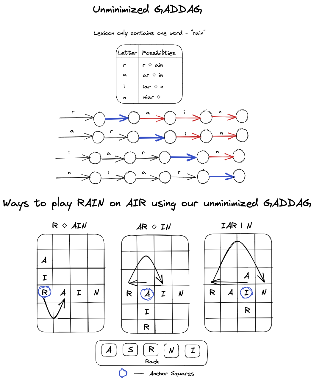
As you can see, each word in the lexicon is created by placing letters leftwards from the anchor square until a \(\diamond\) is observed. Then, letters are placed to the right of the anchor square until an acceptable word is formed. The paths are explored using a depth-first search approach, backtracking when necessary due to letter availability on the rack or board limitations.

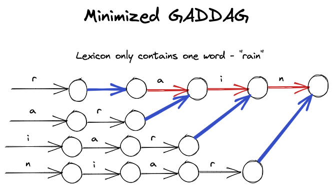
However, as one might notice, an un-minimized GADDAG generates more edges than an un-minimized DAWG. To make it space-efficient, we can optimize it by allowing arcs to connect letters that if encountered next, can form a word. Applying this partial minimization technique would have the following effect on the above GADDAG:

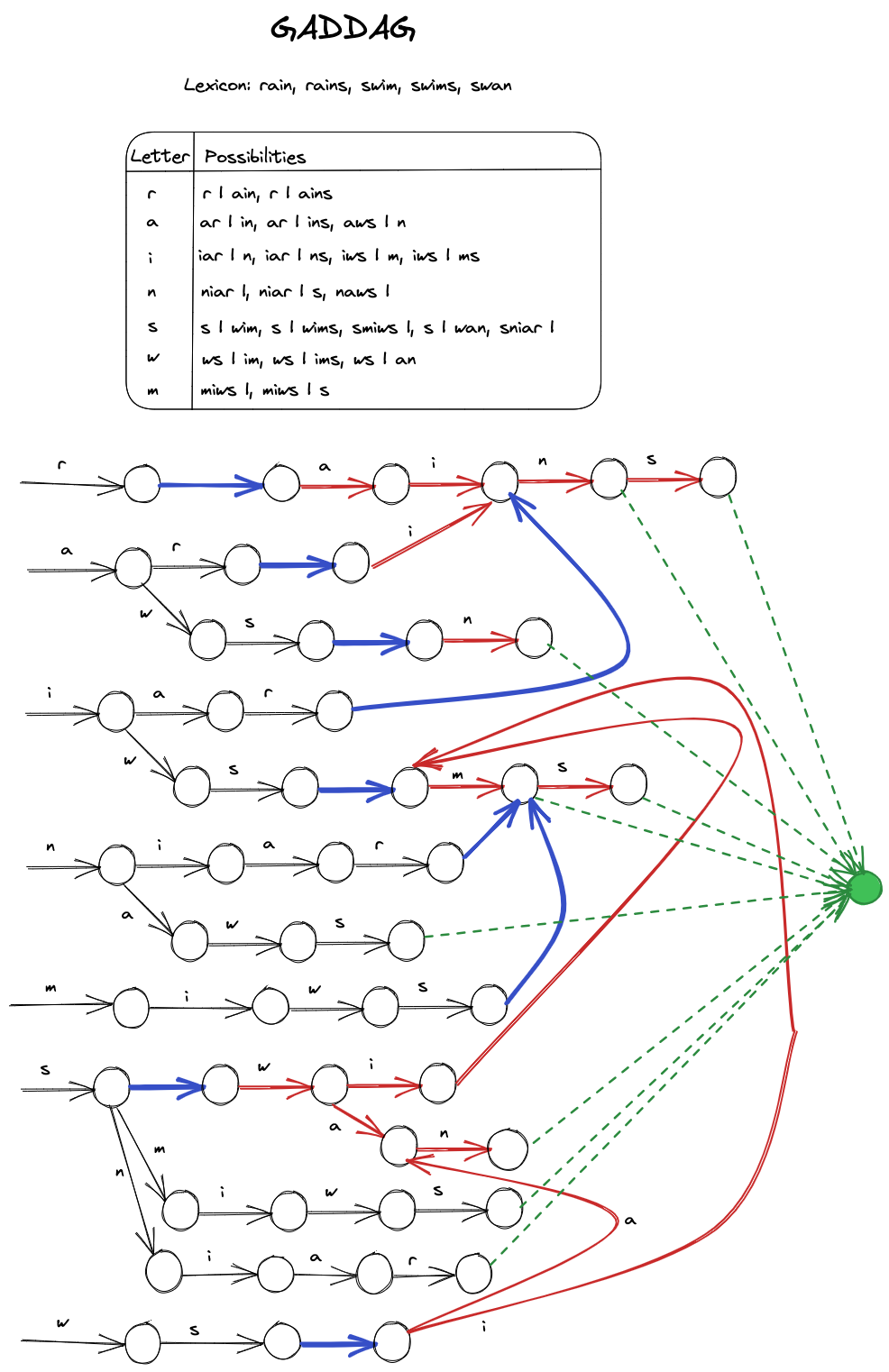
Furthermore, here's a minimized GADDAG for a much larger lexicon consisting of five words.

To generate valid moves from an anchor square using a GADDAG, the following backtracking, recursive algorithm can be used.

Gen\((pos, word, rack, arc)\):
1. If a letter \(L\) is already on this square:
1. \(nextArc = arc \rightarrow L\)
2. GoOn\((pos, L, word, rack, nextArc, arc)\)
2. Else if letters remain on \(rack\):
1. For each letter \(L\) on the \(rack\):
1. If letter is allowed on this square (i.e. there can be a potential arc):
1. \(nextArc = arc \rightarrow L\)
2. GoOn\((pos, L, word, rack - L, nextArc, arc)\)

GoOn\((pos, L, word, rack, newArc, oldArc)\):
1. If \(pos \le 0\):
1. \(word = L || word\)
2. If terminal node is reached & no letter directly left:
1. \(word\) is a valid word in the lexicon, can be a possible move
3. If newArc be traversed further:
1. If there is room to the left:
1. Gen\((pos - 1, word, rack, newArc)\)
2. \(nextArc = newArc \rightarrow \diamond\)
3. If \(nextArc\) can be traversed further & no letter directly left & room to the right:
1. Gen\((1, word, rack, nextArc)\)
2. Else if \(pos \gt 0 \):
1. \(word = word || L\)
2. If terminal node is reached & no letter directly right:
1. \(word\) is a valid word in the lexicon, can be a possible move
3. If \(newArc\) can be traversed further & room to the right:
1. Gen\((pos + 1, word, rack, newArc)\)

The Gen function takes the position (\(pos\)) on the board where the move should start, the current word being formed (\(word\)), the letters remaining in the rack (\(rack\)), and the current arc (\(arc\)) being followed as inputs. When initially starting at the anchor square, Gen\((0, Null, Rack, Init)\) is called, where the arc is to the initial state of GADDAG \(Init\).

The algorithm first checks if a letter exists at the current square. If it does, it follows the arc corresponding to that letter (\(newArc\)) and calls itself recursively with the new position.

If there is no letter at the current square, it loops over all the letters in the rack and checks if they can be played on the current square (i.e. if there exists a potential arc). If there is, it follows the arc corresponding to that letter (\(newArc\)) and calls itself recursively with this new position.

When the algorithm finds that the current word is a valid word in the lexicon and that there is no letter immediately preceding/succedding it on the board, the word is added to the list of possible moves.

Throughout, GoOn checks if the new arc can be traversed further and if there is room to the left or right to continue forming the word. If there is, the algorithm follows the new arc and calls itself recursively with the new position.

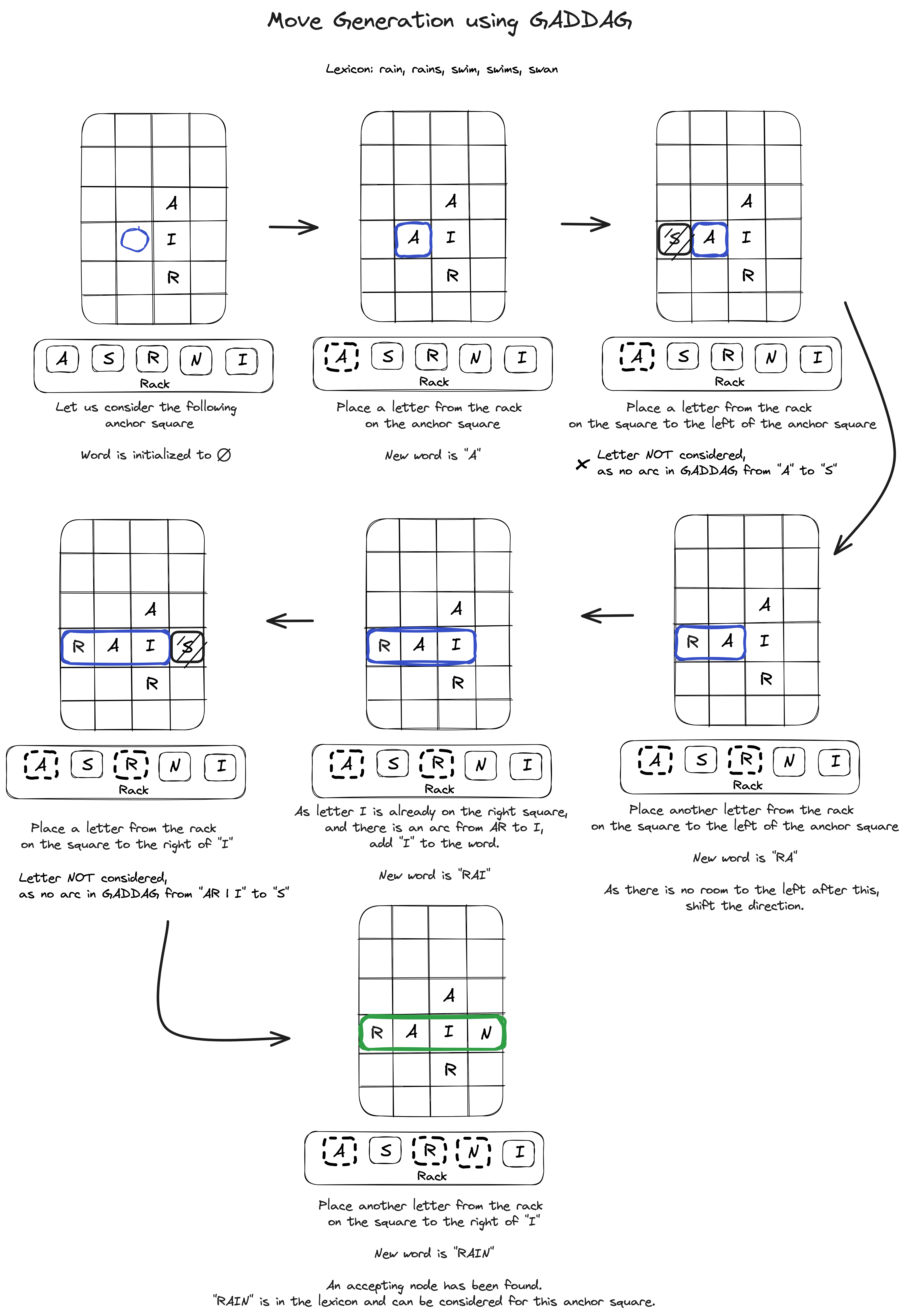
The Figure 10 shows a step-by-step process of how the GADDAG from Figure 9 can be used to generate moves from a particular anchor square.

In his performance analysis, Gordon shows how GADDAGs can generate moves twice as fast as DAWGs. However, they can take up to five times as much memory for a typical-sized lexicon. We won't be delving into these analyses, but we encourage curious readers to read his paper.

←