KHyperLogLog
The Secret World of Data Structures and Algorithms, Chapter 1
Author: Parth Parikh
First Published: 24/01/23
Truth is much too complicated to allow anything but approximations. - John Von NeumannI have always dreamed of writing a short book on data structures and algorithms that are not widely known outside of academic circles. My initial goal was to complete it before I turned 30, but then I thought, "Why wait? Carpe diem!" This is the draft of the first chapter. I plan to open-source all eight chapters of my book. This is my first time pursuing such an adventure, and I would greatly appreciate your feedback.
This chapter discusses KHyperLogLog, an algorithm introduced by Google that is based on approximate counting techniques that can estimate certain privacy risks of very large databases using linear runtime and minimal memory.
Introduction
In the mid-90s, the Massachusetts Group Insurance Commission (GIC) released data on state employees' hospital visits, claiming it was anonymized. However, Latanya Sweeney, a Ph.D. student at MIT at the time, discovered that by linking the medical data with the voter roll in Cambridge, some data could be de-anonymized. To the surprise of many, Sweeney was able to successfully identify then Massachusetts governor, William Weld, in relation to his medical records.
Paul Ohm, a Professor of Law at Georgetown University, recalled this incident in his paper titled “Broken Promises of Privacy”:
At the time that GIC released the data, William Weld, then−Governor of Massachusetts, assured the public that GIC had protected patient privacy by deleting identifiers. In response, then−graduate student Sweeney started hunting for the Governor’s hospital records in the GIC data. She knew that Governor Weld resided in Cambridge, Massachusetts, a city of fifty-four thousand residents and seven ZIP codes. For twenty dollars, she purchased the complete voter rolls from the city of Cambridge—a database containing, among other things, the name, address, ZIP code, birth date, and sex of every voter. By combining this data with the GIC records, Sweeney found Governor Weld with ease. Only six people in Cambridge shared his birth date; only three were men, and of the three, only he lived in his ZIP code. In a theatrical flourish, Dr. Sweeney sent the governor’s health records (including diagnoses and prescriptions) to his office.
Later, in the year 2006, AOL released approximately 20 million search queries from 650,000 users collected over three months, with the intent of allowing researchers to understand search patterns. They anonymized the records by removing user identifiers and released the data with the following attributes: AnonymousID, Query, QueryTime, ItemRank, and ClickURL.
A few days later, two New York Times journalists, Michael Barbaro and Tom Zeller Jr. began investigating the search queries and discovered that a user with the anonymous ID 4417749 had queried for things like landscapers in Lilburn, GA, people names with last name Arnold, and homes sold in shadow lake subdivision gwinnett county georgia.
By narrowing down the search to 14 citizens with the last name Arnold near Lilburn, GA, they were able to identify the user as 62-year-old Thelma Arnold! This led to a class-action lawsuit being filed against AOL, which was eventually settled in 2013.
These incidents highlight the ease with which seemingly anonymized data can be de-anonymized. In an ideal world, organizations would employ mitigation techniques to ensure that such linkage attacks cannot occur, both within the organization and when the data is publicly released.
However, comprehending the privacy risks associated with data can be a challenge, especially for large organizations that handle vast amounts of information. It raises the question, how can we automate and scale the process to accommodate large databases? This is the central issue we will be addressing in this chapter.
Let us begin by discussing two characteristics of data sets that can aid in these privacy assessments - reidentifiability and joinability.
To understand these concepts, let us consider an example of a medical database with attributes such as Social Security Number, Date of Birth, Gender, ZIP code, and Diagnosis. Even if sensitive information like the Social Security Number is removed from this database, it can still be vulnerable to a linkage attack by using auxiliary data such as Date of Birth, Gender, and ZIP code from voter information, as demonstrated by Dr. Sweeney in the Cambridge de-anonymization case.
Reidentifiability is a characteristic that measures the potential for a given anonymized or pseudonymized data to be de-anonymized, revealing the identities of the users.
Joinability is another characteristic that measures whether two or more datasets can be linked by unexpected join keys, such as Date of Birth, Gender, and ZIP code in our example.
The KHyperLogLog algorithm, which will be the focus of this chapter, is an algorithm introduced by Google that helps estimate the risks of reidentifiability and joinability in large databases.
Approximate Counting
To understand KHyperLogLog, we must first delve into the concept of Approximate Counting. Simply put, approximate counting is a technique that approximates the number of distinct elements in a set by using a small amount of memory.
There are two common algorithms for approximate counting: K Minimum Values (KMV) and HyperLogLog (HLL).
K Minimum Values
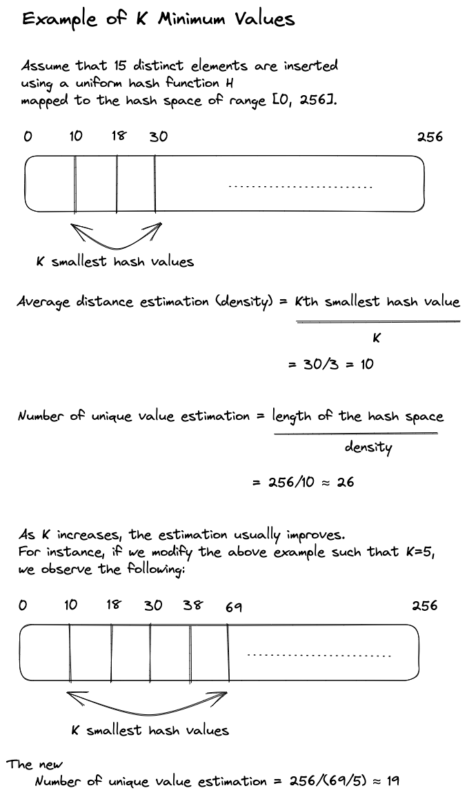
K Minimum Values (KMV) estimates the number of distinct elements (N) in a set by keeping track of the K smallest hash values of the elements. It has a time complexity of O(N) and a space complexity of O(K).
The intuition behind KMV is that if we assume we have a hash function H whose output is evenly distributed across the hash space, we can estimate the number of distinct elements by computing the average distance between two consecutive hashes (referred to as the density) and then dividing the length of the hash space by this density.
However, even for 32-bit hashes, the storage cost can be substantial if the number of distinct elements is large. To overcome this, KMV uses the K smallest hash values to extrapolate the density of the hash space. An example of this is shown in Figure 1.
The estimations produced by K Minimum Values algorithm have a relative standard error rate of √ 1/K . For example, if K = 1024 and the hash function generates 64-bit hashes, then the relative standard error rate of the estimations is 3.125% and the size of KMV is 8 KB (1024 * 8 bytes).
HyperLogLog
Instead of keeping track of the K smallest hash values and computing the average distance estimation, we can keep track of the maximum number of trailing zeros seen from all the hash values. This, as we will observe, will help reduce space complexity.
The intuition behind this approach is that, given the uniformity assumption of our hash function, as the number of distinct elements seen by us increases, the maximum number of trailing zeros seen also increases. We can then use this idea to extrapolate the approximate count. This concept is perfectly explained by Salvatore Sanfilippo, the author of Redis, an in-memory database that supports HyperLogLog:
Imagine you tell me you spent your day flipping a coin, counting how many times you encountered a non interrupted run of heads. If you tell me that the maximum run was of 3 heads, I can imagine that you did not really flipped the coin a lot of times. If instead your longest run was 13, you probably spent a lot of time flipping the coin.
However if you get lucky and the first time you get 10 heads, an event that is unlikely but possible, and then stop flipping your coin, I’ll provide you a very wrong approximation of the time you spent flipping the coin. So I may ask you to repeat the experiment, but this time using 10 coins, and 10 different piece of papers, one per coin, where you record the longest run of heads. This time since I can observe more data, my estimation will be better.
Long story short this is what HyperLogLog does: it hashes every new element you observe. Part of the hash is used to index a register (the coin+paper pair, in our previous example. Basically we are splitting the original set into m subsets). The other part of the hash is used to count the longest run of leading zeroes in the hash (our run of heads). The probability of a run of N+1 zeroes is half the probability of a run of length N, so observing the value of the different registers, that are set to the maximum run of zeroes observed so far for a given subset, HyperLogLog is able to provide a very good approximated cardinality.
More formally, when working with a hash of P bits, we utilize the first X bits to index into the register, and the remaining P-X bits to count the maximum number of trailing zeros at that register. This approach results in the creation of 2X such registers, ensuring a space complexity of O(2X).
After the stream of data elements is observed, HyperLogLog estimates the number of distinct elements in each register (BI) as 2I, where I represent the maximum number of trailing zeros seen in register I. The overall estimation of unique values is determined by taking the harmonic mean of BI for all values of I.
But why use the harmonic mean instead of the geometric mean? The authors of HyperLogLog explained in their paper that:
The idea of using harmonic means originally drew its inspiration from an insightful note of Chassaing and Gérin: such means have the effect of taming probability distributions with slow-decaying right tails, and here they operate as a variance reduction device, thereby appreciably increasing the quality of estimates.
Intuitively, this means that the harmonic mean helps reduce the impact
of unusually large trailing zero counts (outliers). For instance, the
harmonic mean of {1,2,2,3,3,9} is 2.16, whereas its
geometric mean is 2.62. Additionally, the harmonic mean
tends to ignore numbers as they approach infinity
- the harmonic mean of {2, 2} = {1.5, 3} = {1, inf} = 2.
In comparison to KMV, HyperLogLog has a relative standard error rate of 1.04/ √ M , where M = 2X. This means that if M = 1024 and the hash function again generates 64-bit hashes, then the relative standard error rate of the estimations is slightly increased to 3.25%, however the size of is drastically reduced to 768 B (assuming each register is of size 6 bits, 1024*6 = 6144 bits = 768 bytes).
KHyperLogLog
Now, let us understand how these approximate counting algorithms can assist us in measuring reidentifiability and joinability.
Before proceeding, it is important to understand that possessing only
cardinality estimates is not helpful. Consider a scenario where we are
storing User Agents along with their corresponding user IDs. A User
Agent on Google Chrome, for example, would look like the following:
Mozilla/5.0 (X11; Linux x86_64) AppleWebKit/537.36 (KHTML, like Gecko) Chrome/51.0.2704.103 Safari/537.36
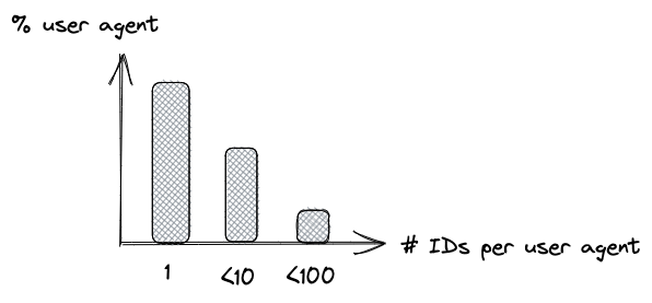
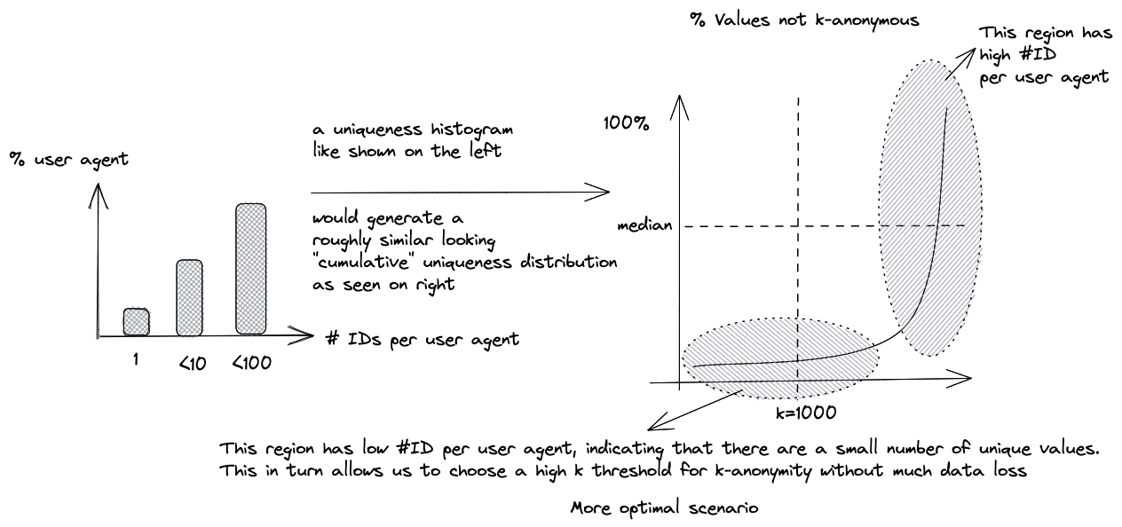
When assessing reidentifiability, we are not particularly interested in the number of unique User Agents we have seen. Instead, we would like to estimate the uniqueness distribution of these User Agents given their user IDs. This would help us understand how many User Agents have unique user IDs, which in turn would increase their chances of getting reidentified. For example, refer to Figure 2.
To estimate such uniqueness distributions, the
KHyperLogLog algorithm
was introduced. It combines the K Minimum Values and HyperLogLog
algorithms into a two-level data structure that stores data of
the type (field, ID). Using our previous example, the
field would be the User Agent, and the
ID would be the user ID.
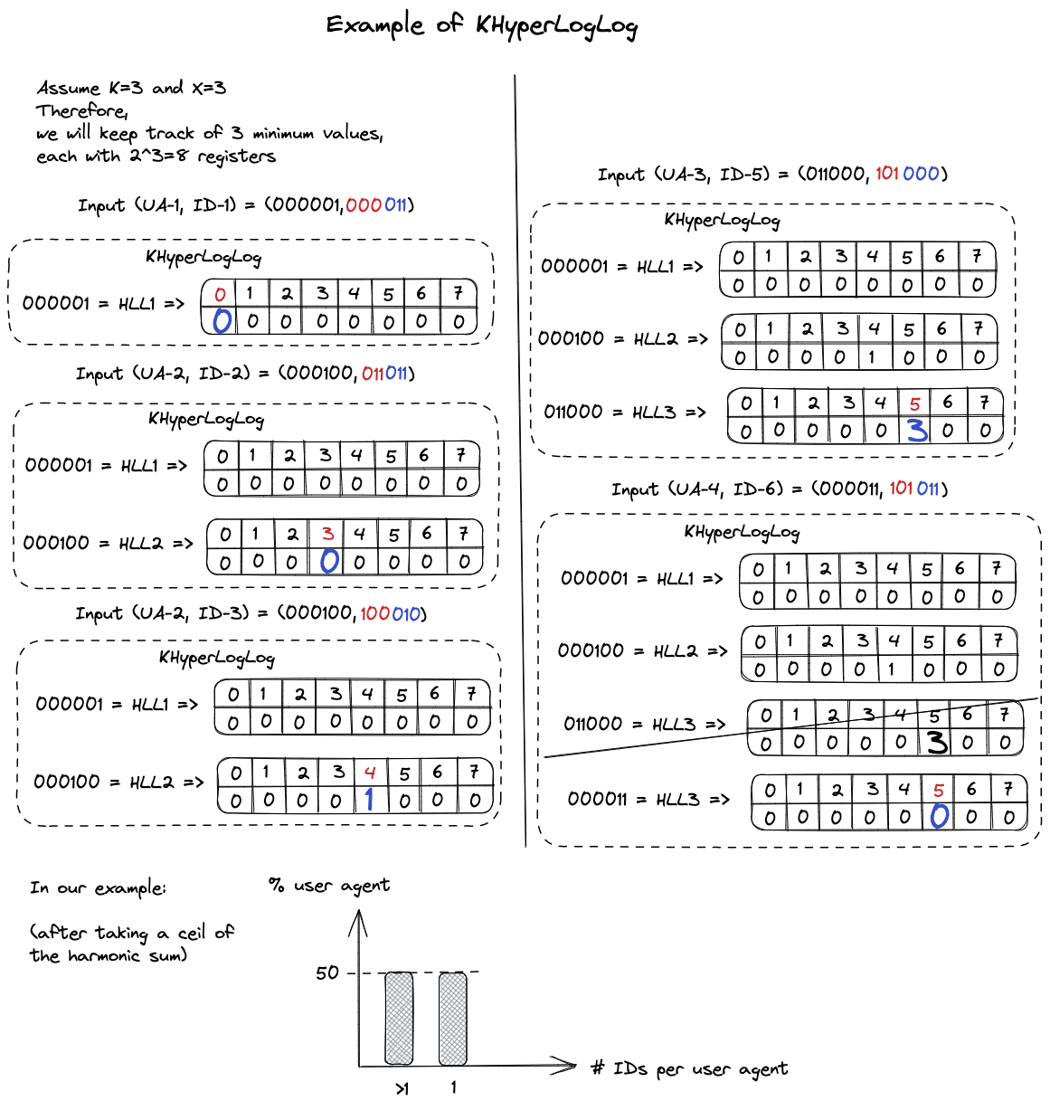
The first level of KHyperLogLog stores the K smallest hashes of field values. Each of these hashes corresponds to a HyperLogLog structure that contains the hashes of IDs associated with their field value and their trailing zero counts.
For a stream of (field, ID) pairs, the
construction algorithm
is as follows:
- Calculate the
h(field)and theh(ID). -
If the
h(field)is present inside the KHyperLogLog data structure (i.e. it is one of the K smallest hashes of field values seen so far), then use theh(ID)to update the HyperLogLog part corresponding toh(field). -
If
h(field)is not present in the KHyperLogLog data structure, check if it belongs among the K smallest hashes. - If it does, proceed to the next step.
- Check if there are more than K entries in the K Minimum Values structure, and if so, remove the entry with the largest hash value.
-
Add the new
h(field)to the K Minimum Values structure, and add theh(ID)to its corresponding HyperLogLog part. - Else, do nothing.
An example of such a construction is provided in Figure 3.
To understand the estimation of reidentifiability using KHyperLogLog, it is essential to first understand the concept of k-anonymity.
k-anonymity
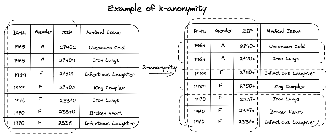
k-anonymity is a technique that prevents linkage attacks by modifying values in such a way that no individual is uniquely identifiable from a group of at least k or more. The value of k represents the degree of anonymity, and such groups form an equivalence class.
One of the methods used to achieve k-anonymity is called Generalization.
This technique involves replacing specific values with generic and
semantically similar values. For example, ZIP codes such as
{13053, 13058, 13063, 13067} can be generalized into
{1305*, 1306*}. Additionally, categories such as
{widowed, married, divorced} can be generalized into
{been_married}.
An example of k-anonymity in action is illustrated in Figure 4.
The general rule of thumb is that: The more generalization you perform, the more information is lost (and thus, the less utility). Therefore, it is recommended to not generalize more than what is necessary.
k-anonymity is a valuable tool in protecting against membership disclosure, which refers to the ability to determine whether an individual is present in a dataset. Another type of disclosure, sensitive attribute disclosure, involves the identification of sensitive information such as salary or political affiliation. While k-anonymity alone may not prevent sensitive attribute disclosure, it can be used in combination with techniques like l-diversity.
l-diversity is concerned with ensuring diversity in sensitive attributes within each equivalence class. In other words, it is important for the sensitive attributes to vary among individuals in the same group. Though we will not delve deeply into l-diversity in this chapter, it is useful to visualize this concept using the above example.
If the second row would also contain Uncommon cold, then one could deduce that someone matching the first three columns has Uncommon cold. However, if we stipulate that the second row must contain a different value for the Medical Issue attribute, then we can ensure that this attribute is not disclosed for a person with the same birth year, gender and ZIP code.
k-anonymity has a direct impact on reidentifiability. When the k value is high, there is more generalization, which in turn increases anonymity and decreases the potential for reidentifiability.
Lastly, it is important to note that k-anonymity is not a highly robust privacy definition. If you desire to securely anonymize your data, more powerful tools such as Differential Privacy may be beneficial.
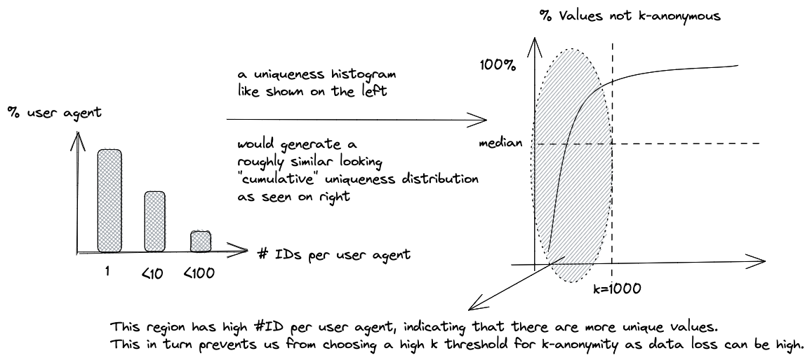
Reidentifiability Estimation
Let us now return to the topic of estimating reidentifiability using KHyperLogLog. Figures 5 and 6 demonstrate how Figure 2 can be modified to estimate a good k threshold. We can then set up periodic analyses to monitor whether the uniqueness is below a given threshold or not.
Joinability Estimation
The joinability of two fields, say F1 and F2 (for instance, User Agents from two databases), can be estimated using a metric called containment.
The containment of F1 in F2 is defined as |F1 ∩ F2| / |F1|. This is different from Jaccard Similarity, which is usually defined as |F1 ∩ F2| / |F1 U F2|. Jaccard Similarity is not ideal in cases where one dataset contains a small subset of users from a larger dataset, as the Jaccard Similarity would be quite low for such cases, even though the containment of the smaller dataset in the larger one would be high.
To compute containment using KHyperLogLog, we require the cardinality of F1, F2, and their intersection. The cardinality of their intersection can be computed using the inclusion-exclusion principle, i.e. |F1 ∩ F2| = |F1| + |F2| - |F1 U F2|.
The union of F1 and F2 can be estimated by merging the KHyperLogLogs of F1 and F2. This can be done by finding the set union of their K Minimum Values structures; that is, by combining the two structures and retaining their K smallest hashes. If F1 and F2 have different K values, we use the smallest K.
Furthermore, we can use F1 and F2's individual K Minimum Value structures to estimate the number of distinct elements in them.
Once we know how to calculate the containment metric, we can create periodic KHyperLogLog-based joinability analyses that check whether the containment score is below an optimal threshold or not.
This strategy has proven to be quite useful for Google, who mentioned how this metric was able to mitigate a significant joinability risk:
Periodic KHLL-based joinability analyses have enabled us to uncover multiple logging mistakes that we were able to quickly resolve. One instance was the exact position of the volume slider on a media player, which was mistakenly stored as a 64-bit floating-point number. Such a high entropy value would potentially increase the joinability risk between signed-in and signed-out identifiers. We were able to mitigate the risk by greatly reducing the precision of the value we logged.
However, care must be taken as this method is still susceptible to false
positives and negatives. For example, one could determine that the
port_number and seconds_till_midnight fields
are joinable since they both have an extensive overlap in the [0, 86400)
value region. Additionally, this metric would fail to detect fields that
have different encodings (such as base64 and raw string) or have
undergone a minor transformation (like a microsecond timestamp and a
millisecond timestamp). Experimentally, it was also noticed that the
containment metric can be unreliable when dealing with highly unequal
set sizes. User intervention is necessary for such scenarios.
Distributed Workflow
The process of generating KHyperLogLog structures for different(field, ID) tuples can be done in a distributed fashion. See
Figure 7 for an illustration of the workflow.
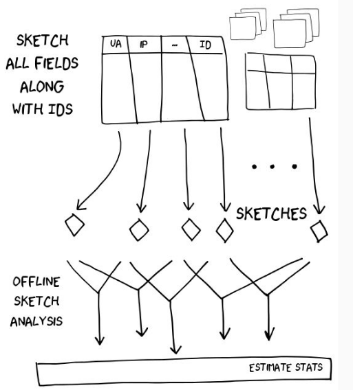
(field, ID) tuples. Then in step 2, periodic
analyses of the thresholds generated from these structures can be done
offline.
Conclusion
In conclusion, KHyperLogLog can be very effective in estimating reidentifiability and joinability at scale in an offline fashion. This, in turn, can help in evaluating privacy strategies surrounding your data and enable efficient regression testing.
Thanks to Damien Desfontaines for reading and improving this chapter.
←