Odd Sketches
The Secret World of Data Structures and Algorithms, Chapter 2
Author: Parth Parikh
First Published: 19/02/23
“Then you should say what you mean," the March Hare went on.Welcome to the draft of the second chapter of my journey to write a short book on data structures and algorithms that are not widely known outside of academic circles. The first chapter discussed KHyperLogLog, an algorithm introduced by Google that is based on approximate counting techniques that can estimate certain privacy risks of very large databases using linear runtime and minimal memory. I'm looking forward to your feedback, which is greatly appreciated.
"I do," Alice hastily replied; "at least-at least I mean what I say-that's the same thing, you know."
"Not the same thing a bit!" said the Hatter. "Why, you might just as well say that 'I see what I eat' is the same thing as 'I eat what I see'!"
"You might just as well say," added the March Hare, "that 'I like what I get' is the same thing as 'I get what I like'!"
"You might just as well say," added the Dormouse, which seemed to be talking in its sleep, "that 'I breathe when I sleep' is the same thing as 'I sleep when I breathe'!"
"It is the same thing with you." said the Hatter,”
― Lewis Carroll, Alice in Wonderland
Introduction
The advent of the World Wide Web in the 1990s is a remarkable feat of engineering. In 1990, Tim Berners-Lee launched the first website and web server, along with the first web browser, WorldWideWeb. Also in the same year, Alan Emtage created the first internet search engine, Archie, marking the start of a new era in technological advancements.
The emergence of the internet brought with it unique challenges for search engines. Early search engines, including Lycos, Netscape, Yahoo, Alta Vista, and later Google, had to devise algorithms for crawling and parsing the rapidly expanding web, devise indexing methods, and create efficient search algorithms. Furthermore, they faced the challenge of building streamlined, distributed systems to handle the immense load while combating spam and ensuring the authenticity of search results.
In this chapter, we will delve into a problem specific to search engines: efficiently estimating the similarity between two sets. To begin, we will examine the Jaccard similarity coefficient. Then, we will explore minhashing, a widely used method for estimating the Jaccard similarity. In doing so, we will uncover an issue with minhashing and how Michael Mitzenmacher, Rasmus Pagh, and Ninh Pham developed a solution for it through the creation of odd sketches almost two decades later.
Jaccard Similarity
The history of Jaccard Similarity is both intriguing and enlightening. In the late 19th century, the United States and several European nations were focused on developing strategies for weather forecasting, particularly for storm warnings. In 1884, Sergeant John Finley of the U.S. Army Signal Corps conducted experiments aimed at creating a tornado forecasting program for 18 regions in the United States east of the Rockies. To the surprise of many, Finley claimed his programs were 95.6% to 98.6% accurate, with some areas even achieving a 100% accuracy rate. Upon publishing his findings, Finley's methods were criticized by contemporaries who pointed out flaws in his verification strategies and proposed their solutions. This sparked a renewed interest in weather prediction, which is now referred to as the "Finley Affair."
One of these contemporaries was Grove Karl Gilbert. Just two months after Finley's publication, Gilbert pointed out that, based on Finley's strategy, a 98.2% accuracy rate could be achieved simply by forecasting no tornado warning. Gilbert then introduced an alternative strategy, which is now known as Jaccard Similarity.
So why is it named Jaccard Similarity? As it turns out, nearly three decades after Sergeant John Finley's tornado forecasting program in the 1880s, Paul Jaccard independently developed the same concept while studying the distribution of alpine flora:
The ratio of the number of species common to two districts (T and D for example) to the total number of species collected in the two districts together (T + D), i.e., their coefficient of community, varies in the three cases given in the table between 50 and 60 per cent.
Thus in spite of their proximity and the similarity of their ecological conditions, the florulae of our three districts possess very different compositions, and the comparative study of these (Number of species common to the two districts X 100)/(Total number of species in the two districts florulae) shows that a great number of common species with a distribution through the entire chain of the Central Alps are actually absent over considerable stretches of country, while the conditions apparently capable of assuring their existence are everywhere realised.
More formally, Jaccard Similarity is defined as the ratio of the cardinality of the intersection of two sets, \( A \) and \( B \), to the cardinality of their union, that is, \( |A \cap B| / |A \cup B| \). When the two sets are identical, the Jaccard Similarity is one, but when they are completely disjoint, it is zero.
What is the time and space complexity of computing this coefficient? Well, if we assume that the size of \( A \) and \( B \) are the same (say \( n \)), we can start by inserting all the elements of \( B \) in a binary search tree-like representation. Then, for each element in \( A \), we can search for that element inside \( B \)’s binary search tree in \(O(\log n)\) time. If an element is found, we increment the intersection and union count by 1, else we only increment the union count by 2. Such an approach can produce an \(O(n \log n)\) time complexity with an \(O(n)\) space complexity. We can certainly do better by inserting the elements of B in a hash table.
However, it becomes evident that for large enough values of \(n\), these methods may not be feasible. This is where the motivation for finding an approximation of the Jaccard Similarity arises. Minhashing is one such technique.
Minhashing
Before the public release of Alta Vista in 1995, its engineers encountered a problem: the search engine was producing highly repetitive results, with the same answers being repeated multiple times. Apparently, this was a significant issue when searching for UNIX manual pages, as back then, tools were used to convert UNIX manual pages into web pages, and these pages often included the institution name and current date, creating multiple copies of the same manual page within the corpus. As these duplicates did not add any value to the user beyond the first copy, they had to be removed from the search results.
To do this, they needed a hashing technique that could flag near-duplicate web pages at scale. What they came up with is a variant of locality-sensitive hashing, which we today know as minhashing. In this section, we are going to look into minhashing in more detail. At a high level, visualize it as a distance measure that estimates the similarity between a pair of documents.
To better understand minhashing, let us examine a characteristic matrix, which provides a visual representation of a collection of sets. For example, with four sets \( S1=\{a, b, d\} \), \( S2=\{c, d, e\} \), \( S3=\{a\} \), and \( S4=\{b, c, d, e\} \), the characteristic matrix would appear as follows:
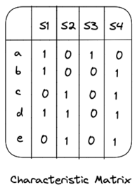
Due to the sparse nature of these matrices, they are not efficient for data storage. However, they will play an important role in visualizing the minhashing technique.
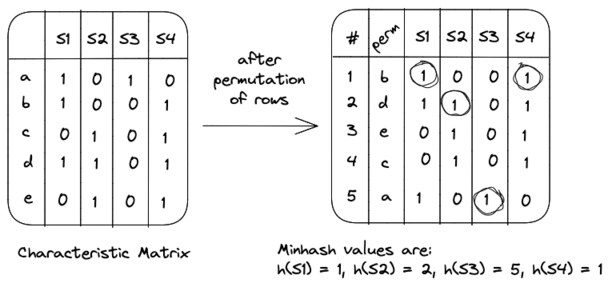
To compute the minhash value of a set (denoted as \(h\)), we start by selecting a random permutation of the rows in the characteristic matrix. For example, a random permutation of \(\{a, b, c, d, e\}\) might be \(\{b, d, e, c, a\}\). The minhash value of a set \(S\) is then determined by the position of the first row in the permuted order in which the corresponding column has a value of 1.
For instance, if we consider the characteristic matrix shown above, the minhash values for the sets would be:
By using multiple permutations (typically 100 or more), we can create multiple hash signatures for each column. For instance, if we extend the previous example with three permutations, the hash signatures would look something like the following:
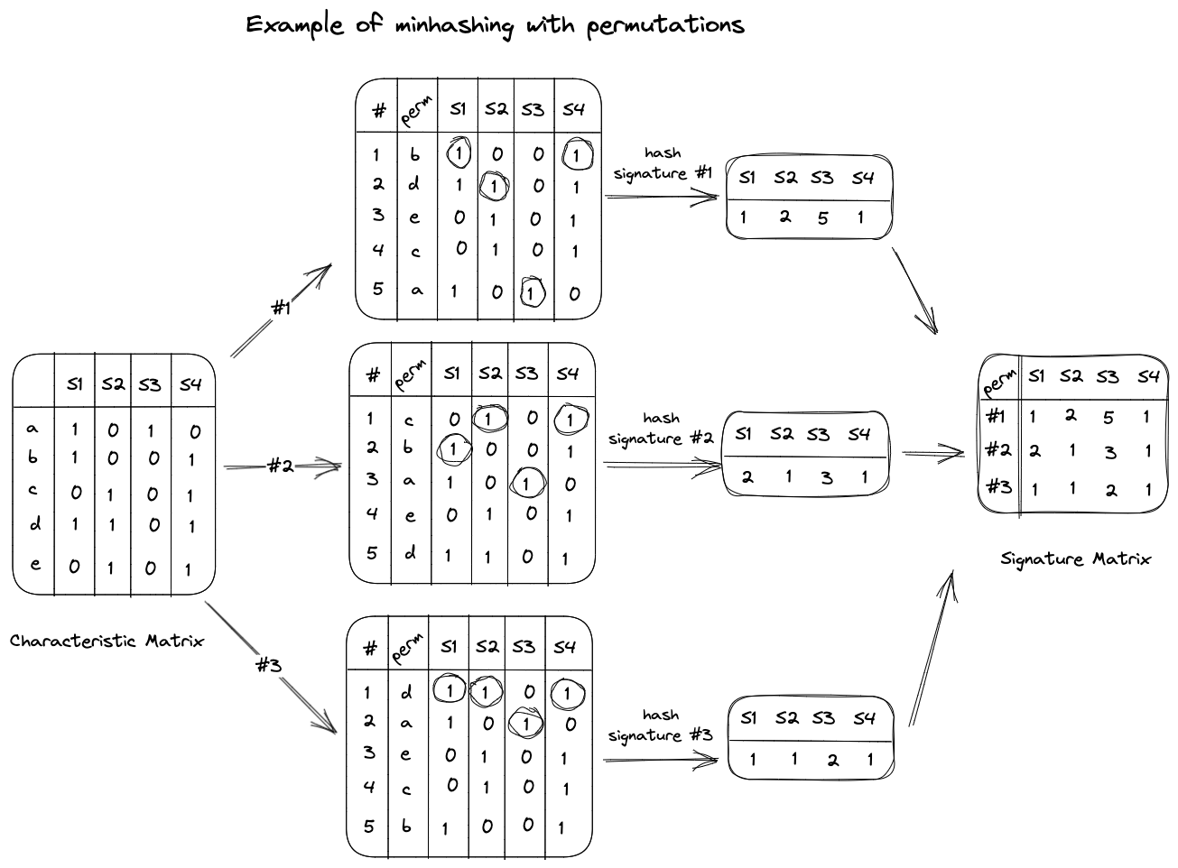
In this manner, we generate a signature matrix that summarizes the minhash values for all our random permutations. We can then estimate the similarity of any two sets by calculating the Jaccard similarity of their respective columns in the signature matrix. For instance, the similarity of sets \(S_2\) and \(S_4\) is estimated to be \(2/3\) or 0.67, as the second and the third permutations have the same hash signature, however, the first one differs. Moreover, if we examine the characteristic matrix, we see that the actual Jaccard similarity between \(S_2\) and \(S_4\) is 0.75. Considering that we only used 3 permutations, 0.67 is a reasonable approximation.
A common question that arises at this stage is, why use random permutations? Why is the minhash value of a set equivalent to the number of the first row in the permuted order? It turns out, for a given random permutation, the probability of the minhash function producing the same value for two sets is equal to the Jaccard similarity of those sets.
This surprising result can be explained as follows:
For any two sets \(S_i\) and \(S_j\), the characteristic matrix has three types of rows:
- Rows with 1 in both columns (x)
- Rows with 1 in one column and 0 in another (y)
- Rows with 0 in both columns (z)
The total number of rows is \( x + y + z \), and the Jaccard similarity of \( S_i \) and \( S_j \) is \( x/(x+y) \), as \(x\) represents the size of the intersection of \( S_i \) and \(S_j\), and \( x + y \) represents the size of the union of \( S_i \) and \( S_j \).
For a random permutation, if we proceed from the top, the probability that we encounter a row with 1 in both columns is \( x/(x+y) \), which is equal to the Jaccard similarity of \( S_i \) and \( S_j \). On the other hand, if we encounter a row with 1 in one column and 0 in another, the minhash values for \( S_i \) and \( S_j \) will differ. Hence, the probability that the minhash function produces the same value for two sets equals the Jaccard similarity of those sets.
While the minhashing technique is conceptually sound, it becomes impractical when applied to a large characteristic matrix, such as one with a billion rows. Generating a random permutation for such a matrix can be time-consuming and accessing rows in the permuted order can cause thrashing.
To address these issues, it's recommended to simulate the effect of \( n \) random permutations using \( n \) random hash functions \((h_1, h_2, … h_n)\). These hash functions should map the row numbers (from 1 to \(k\)) to bucket numbers within the same range (1 to \(k\)) with minimal collisions. This is achievable if the range \(k\) is large enough.
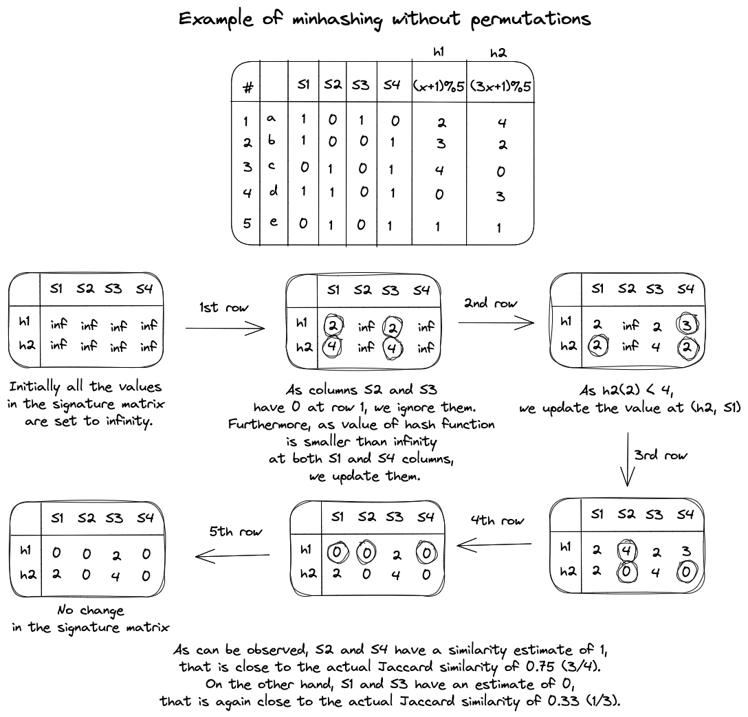
The signature matrix consists of \( n \) rows and the same number of columns as the characteristic matrix. To construct such a matrix, we process each row, \( r \), as follows:
- Compute \(h_1(r), h_2(r), … h_n(r)\).
- For each column, \(c\):
- If \(c\) has 0 in row \(r\), do nothing.
- Else, if \(c\) has 1 in row \(r\), then for each hash function, \(h_i\), from 1 to \(n\):
- If \(h_i(r)\) is smaller than the value at the corresponding position in the signature matrix, update that position with \(h_i(r)\).
An example of this construction is shown in Figure 4.
Additionally, to further increase efficiency, one can consider only the first \(m\) rows out of \(k\). The computation can also be made parallel by dividing the \(k\) rows into \(p\) sections, parallelly computing signature matrices for each section, and taking their average. For those interested in exploring these methods in more detail, we recommend reading sections 3.3.6 and 3.3.7 of the "Mining of Massive Datasets" textbook.
To improve the space efficiency of minhashing, Ping Li and Arnd König developed a popular variant known as \(b\)-bit minhashing, where instead of storing \(b=64\) or \(b=32\) bits for each integer in the signature matrix, we would store only the lowest \(b\) bits. The intuition is that the same hash values would give the same lowest \(b\) bits, whereas the different hash values would give different lowest \(b\) bits with a probability of \(1 - 1/2^b\).
We can calculate this probability by first noting that the probability of the lowest 1 bit having the same value is \(1/2\). Moreover, the probability of the lowest 2 bits having the same values is \(1/4\) or \(1/2^2\). Therefore, the probability of the lowest \(b\) bits having the same value would be \(1/2^b\), and for them to be different, the probability would have to be \(1 - 1/2^b\).
However, Mitzenmacher, Pagh, and Pham showed that when the Jaccard similarity is high, this \(b\)-bit minhashing scheme would offer less information than it might be able to. For instance, if the similarity estimate from the \(b\)-bits gives a perfect 1 (i.e. all of the lower bits are identical), we cannot be too confident that the Jaccard similarity is exactly 1. Even a difference of a few flipped bits in the upper bits can lead to very different conclusions for \(J = 1\), especially so when the lower bits are highly correlated. Such precision is especially important when ranking the most similar documents out of hundreds of thousands of documents based on their Jaccard similarity coefficient.
So how do we do this? How do we keep the niceties of minhashing intact, while also reducing the space complexity and increasing the accuracy when estimating sets of high similarity? As it turns out, odd sketches is just the solution for this.
Odd Sketches
Streaming algorithms handle large data streams by using a compact data structure called a sketch. These sketches summarize the data while consuming much less memory than what would be theoretically required to store all the data. An example of a sketch is the HyperLogLog data structure introduced in Chapter 1.
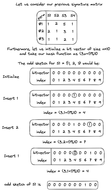
An odd sketch is also a sketch that is constructed using the minhashes of a particular set. It consists of a bit vector of size \(n > 2\) bits which is initialized with zeros.
Assume that we have a column of a signature matrix (\(S\)) that represents the minhash of a particular set in the matrix. Then, the construction of an odd sketch would be as follows:
- Initialize a bit vector \(s\) of size \(n > 2\) bits with zeros. This will store our odd sketch
- Pick a random hash function \(h\) that maps elements to a codomain of range 0 to \(n\)
- For each element \(x \in S\) do
- \(s_{h(x)} = s_{h(x)} ⊕ 1\)
- Return \(s\)
Extending the example seen before, an odd sketch construction would appear as follows:
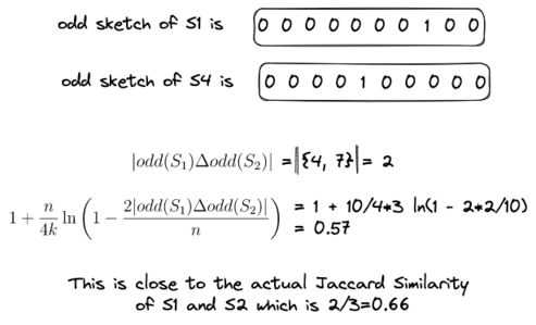
In practice, \(n\) would be much smaller than a signature matrix column's size. After constructing two odd sketches, we can estimate their Jaccard similarity using the following equation: \[ 1 + \frac{n}{4k} \ln \left( 1 - \frac{2 |odd(S_1) \Delta odd(S_2)|}{n} \right) \]
Here, \(k\) denotes the number of independent permutations used during minhashing, and \( odd(S_i) \) represents the odd sketch of a signature matrix column. Additionally, \( odd(S_1) \Delta odd(S_2) \) counts the number of 1s that occur after obtaining the symmetric set difference of the odd sketches of \( S_1 \) and \( S_2 \). It is essential to note that this symmetric set difference is for a multiset. Using this equation, the Jaccard Similarity for the previous example would be:
Although Odd Sketches offer more accurate Jaccard similarity estimates over \(b\)-bit minhashing, there is a small hiccup: in practice, they require more permutations but less storage space than the original minwise hashing scheme. As we discussed in the minhashing section, permutations can be costly. To get the best of both worlds, it's recommended to combine the concepts of minhashing without permutations with odd sketches.
Additionally, we haven't delved into the derivation of the Jaccard similarity estimate. It involves Probability Theory and Statistics, but the Appendix breaks down most of the math behind Odd Sketches in a simpler way for curious readers.
Conclusion
In conclusion, Odd Sketches provide a more accurate Jaccard similarity estimate over \(b\)-bit minhashing while also significantly improving the space complexity over standard minhashing techniques.
Appendix
Analyzing the section on estimating set size from an Odd Sketch
To estimate the size of a column of a signature matrix, which is essentially the number of permutations, we can use the following formula once we have constructed an odd sketch: \[ \frac{-n}{2} \ln(1 - 2z/n) \]
This formula proves to be useful for estimating the Jaccard similarity from odd sketches, as we will see. Here, \(n\) is the size of the odd sketch, and \(z\) is the number of bits with a value of 1.
The derivation of this formula may seem unexpected, so let us delve into how we arrived at it. Suppose that the size of the column of a signature matrix is \(m\), and the size of its corresponding odd sketch is \(n\). Since we used a fully random hash function in the construction, we can think of the process of building our odd sketch as tossing \(m\) balls independently into \(n\) bins. To estimate the size of \(m\), we can use the standard Poisson approximation to the balls-and-bins model.
A discrete random variable \(X\) is said to have a Poisson distribution with parameter \( \mu > 0 \), if its probability mass function is given by: \[ \text{Pr}(X=r) = \frac{\mu^r e^{-\mu}}{r!} \]
To understand this, let's first find the expected fraction of bins with \(r\) balls for any constant \(r\). Let \(X_i\) be a random variable that is 1 when the \(i^{\text{th}}\) bin has \(r\) balls and 0 otherwise. By linearity of expectations, we have: \[ E[X] = E[\sum_{i=1}^{n} X_i] = \sum_{i=1}^{n} E[X_i] \]
The probability that a given bin has \(r\) balls is given by: \[ \binom{m}{r} \left(\frac{1}{n}\right)^r \left( 1 - \frac{1}{n} \right)^{m-r} \]
Here, \( \binom{m}{r} \) indicates that there are \( \binom{m}{r} \) distinct sets of \(r\) balls, \( \left(\frac{1}{n}\right)^r \) indicates that for any set of \(r\) balls, the probability that it lands in this bin is \( \left(\frac{1}{n}\right)^r \), and \( \left( 1 - \frac{1}{n} \right)^{m-r} \) is the probability that it lands in one of the other bins.
Expanding the binomial coefficient on the left side and approximating the right side using Taylor expansion , we get approximately: \[ \frac{1}{r!}\left(\frac{m}{n}\right)^r e^{-m/n} \]
Substituting \( \mu = m/n \), gives the Poisson distribution. The probability that the random variable \(X\) is odd, denoted as \(p\), can be expressed as: \[ \sum_{r\: \text{odd}} \frac{\mu^r e^{-\mu}}{r!} = e^{-\mu} \sum_{r\: \text{odd}} \frac{\mu^r}{r!} = e^{-\mu} \left(\frac{e^{\mu} - e^{-\mu}}{2} \right) = \frac{1 - e^{-2u}}{2} \]
The expansion of \(\mu^r/r!\) can be understood by observing the relationship between hyperbolic functions and the exponential function .
Consider a setting where the number of balls is independently Poisson distributed in each bin with \( \mu = m/n \). Let \( Y_i \) be the parity of the number of balls that land in the \( i^\text{th} \) bin, and let \( Y = \sum_{i=1}^n Y_i \) be the number of bins with an odd number of balls. Then, the expected value of \(Y\) can be expressed as: \[ E[Y] = np = n \left( \frac{1 - e^{-2m/n}}{2} \right) \]
We can approximate \(E[Y]\) to be \(z\), where \(z\) is the number of bins with an odd number of balls in the sketch. Substituting this value into the previous equation, we obtain: \[ m’ = \frac{-n}{2} \ln(1 - 2z/n) \]
Note that to understand the math presented in this section, Michael Mitzenmacher and Eli Upfal's textbook on Probability and Computing can be helpful.
Analyzing the section on estimating Jaccard Similarity from Odd Sketches
For Jaccard Similarity \(J\) and two minhashes \(S_1\), \(S_2\), we can use the formula of \(J\) to determine that \(J = |S_1 \cap S_2|/|S_1 \cup S_2| = |S_1 \cap S_2|/n\). This means that \( |S_1 \cap S_2| = Jn\). Additionally, we can see that \(|S_1 \Delta S_2| = 2(1-J)n\), which represents the white space of the two sets.
If we assume that \(k\) is the number of independent permutations, then we can reformulate the equation as \(|S_1 \Delta S_2| = 2(1-J)k\). This is because the number of independent permutations equals the size of the column of a signature matrix.
Using the equation mentioned in the previous section, we can estimate the set size of \( S_1 \Delta S_2\) as \[|S_1 \Delta S_2| = \frac{-n}{2} \ln(1 - 2|odd(S_1) \Delta odd(S_2)|/n) \] As mentioned in the Odd Sketches section, \(|odd(S_1) \Delta odd(S_2)|\) counts the number of 1s that occur after obtaining the symmetric set difference of the odd sketches of \( S_1 \) and \( S_2 \).
Now substituting \(|S_1 \Delta S_2|\) with \(|S_1 \Delta S_2| = 2(1-J)k\), we can observe that \[ \frac{-n}{2} \ln(1 - 2|odd(S_1) \Delta odd(S_2)|/n) = 2(1-J)k \] \[ \frac{-n}{4k} \ln(1 - 2|odd(S_1) \Delta odd(S_2)|/n) = 1-J \] \[ J = 1 + \frac{n}{4k} \ln \left( 1 - \frac{2 |odd(S_1) \Delta odd(S_2)|}{n} \right) \]
←