If you like this blog post, do subscribe to my RSS feed

Roaring Bitmaps

The Secret World of Data Structures and Algorithms, Chapter 4

Author: Parth Parikh

First Published: 28/02/24

Like a rolling stone
Like a rolling stone
Like a rolling stone
Like the FBI
And the CIA
And the BBC
B.B. King
And Doris Day
Matt Busby, dig it, dig it
Dig it, dig it, dig it
― The Beatles, Dig It

Welcome to the draft on the fourth chapter of "The Secret World of Data Structures and Algorithms". The first three chapters can be explored here. As always, I'm looking forward to your feedback, which is greatly appreciated.

In this chapter, we will journey through the realm of Bitmaps. We will start with Bitmaps and understand what Bitmap indexes are. Then, we will uncover strategies to efficiently compress them, starting with Run Length Encoding (RLE), followed by Byte-Aligned Bitmap Code (BBC), and then venturing deep into the woods with Word-Aligned Hybrid Code (WAH), Compressed 'n' Composable Integer Set (Concise), and finally, Roaring Bitmaps. Happy exploring!

Bitmaps

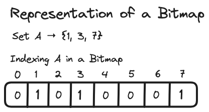
Imagine a bitmap as an array where each element stores either a \(0\) or \(1\). Given that each element can store only two possible values, they can be represented as a single bit. A collection of these elements forms an array, hence it is also referred to as a bit array or binary array.

A bitmap is typically constructed by mapping a domain, such as a range of integers from \([0, n-1]\), to the set {0, 1}. The \(i^{\text{th}}\) bit is set to one if the \(i^{\text{th}}\) integer in the range \([0, n-1]\) is present in the set. This approach naturally results in a compact representation of data, which is often combined with efficient indexing techniques to achieve strong runtime performance with minimal memory overhead.

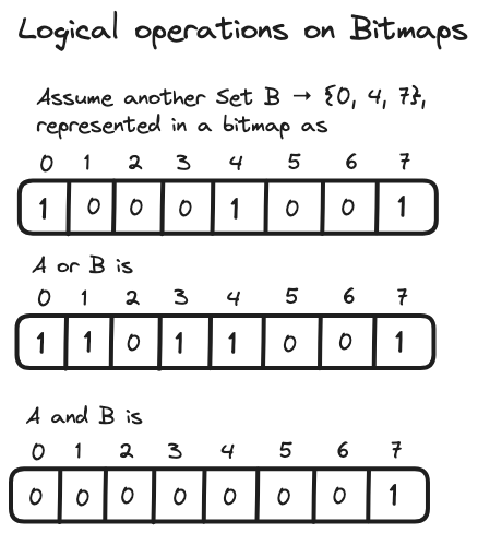
An important aspect of a bitmap is its ability to efficiently perform logical operations. For instance, logical operations on two bitmaps involve comparing corresponding bits from each bitmap and applying a boolean operation (such as AND, OR) to produce a new bitmap. For example, an AND operation sets a bit in the resulting bitmap only if the same position in both original bitmaps is set 1. OR sets a bit if it is set in either of the original bitmaps. These operations allow for efficient combination and intersection of sets, making them useful for analysing data.

Creating a historical narrative from the old seas of research papers is a truly captivating experience. One hopes to dip their feet into the seas enough to savor the waves, but more often than not, we find ourselves drowning, partly due to the awe and majesty of it all. Researching the history of bit maps has been a similar experience for me.

Fascinatingly, APL (A Programming Language), developed by Kenneth Iverson, appears to be one of the earliest programming languages to incorporate the concept of operating on collections of bits as arrays, emphasizing operations on these structures as a fundamental aspect of the language. At that time, what we now refer to as bitmaps were known as logical vectors. In his 1962 paper, Iverson described APL as follows:

The language is broad in scope, having been developed for, and applied effectively in, such diverse areas as microprogramming, switching theory, operations research, information retrieval, sorting theory, structure of compilers, search procedures, and language translation. The language permits a high degree of useful formalism. It relies heavily on a systematic extension of a small set of basic operations to vectors, matrices, and trees, and on a family of flexible selection operations controlled by logical vectors.

Today, this data structure finds myriad applications, including its extensive use in databases, a topic we will explore as we progress through this chapter. Before we do so, let us explore an interesting application that can be found in the Linux kernel’s scheduler.

At its core, the scheduler within the Linux kernel assigns tasks based on the highest priority within the system. When multiple tasks share the same priority level, they are scheduled in a round-robin manner. The role of bitmaps comes into play in identifying this highest priority level and achieving it in constant time.

To do this, the kernel uses a priority array, a form of bitmap, to track the number of active tasks across all priority levels. There are 140 priority levels, 0-99 for real-time processes and 100-139 for normal processes. The system ensures tasks with lower priority numbers take precedence over those with higher numbers. Consider a scenario with four active tasks: two at priority 0, one at priority 100, and another at priority 102. In this case, bits 0, 100, and 102 in the priority array would be set to 1. Consequently, pinpointing the highest priority level in the system is achievable through the find first set (ffs) operation. This involves identifying the first set bit starting from the least significant position. It is possible to do this in constant time, as many CPUs offer specialized instructions for efficiently scanning bits within a register, such as the tzcnt (count trailing zeros) used by x86 processors (supporting Bit Manipulation Instruction Set 1).

One of the approaches to answering queries in the database realm is OLAP (Online Analytical Processing). Think of OLAP as a supermassive library system designed for querying large volumes of data to uncover trends and insights. Unlike looking for specific sections or sentences in a book, OLAP helps you explore broad topics across many books. For instance, imagine that you want to see all discussions related to "Mars missions" across different books to understand trends in space exploration over the years.

Now, sequentially scanning through all the records (book pages in this example), has generally been found to be ineffective. Nevertheless, we can implement optimizations to improve this process. One such optimization could be data prefetching, where we load data blocks or pages into a database’s main memory buffer in advance. This reduces the I/O wait times, and by extension, improves the overall throughput. Another optimization involves multi-threading, where we can have multiple threads scan the data concurrently, thus parallelizing the tasks. Yet another optimization is late materialization, where we stitch the column together as late as possible. Specifically, during a sequential scan to retrieve data, the database often fully constructs each row of the result set early in the process. This means pulling together all the requested columns for a row, even if subsequent operations (like filters or joins) might not require all of this information. Late materialization delays this process by initially working with row identifiers or necessary columns. This helps reduce the volume of data being processed early on. Another optimization over the sequential scans is data skipping - which will serve as a motivation for using bitmaps in database systems.

Data skipping is about identifying data that need not be read ahead of time, allowing us to bypass unnecessary scans at query time. One method to achieve this is through approximate queries, executing them on sampled subsets of the entire table to yield approximate results. Occasionally, a probabilistic data structure can be utilized to store these approximate outcomes. For instance, HyperLogLog is commonly used to estimate the count of unique elements in a list, such as approximating the number of unique views a web page has seen. We have discussed this in greater depth in Chapter 1.

However, these are not the only solutions. Data pruning is another technique, where we rely on an auxiliary data structure, pre-built on our columns, to identify parts of data files in a table that need not be read. And surprise, surprise, one such auxiliary data structure is bitmap indexes.

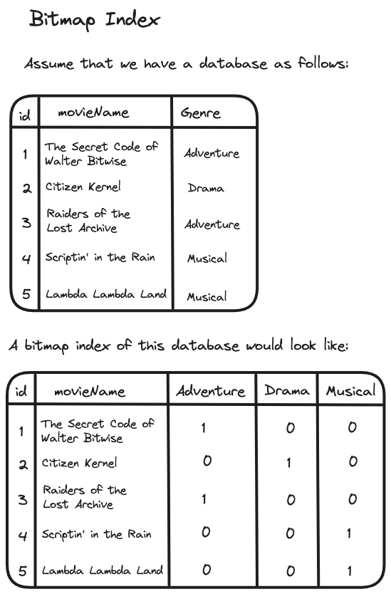
To understand what an “index” is, let us revisit the book analogy, focusing on textbooks. Every textbook you read is likely to have an “Index” or a “Table of Contents” that provides pointers to specific chapters of that book. “Look ‘Space Exploration’ is discussed in chapter 6 on page 458”. Similar to this, databases also have an index that can provide fast access to data items. One of the most common types of these indexes is the primary key index that ensures the unique identification of table rows. In a bitmap index, we store a separate bitmap for each unique value for an attribute where the \(i^{\text{th}}\) position in the bitmap corresponds to the \(i^{\text{th}}\) row in the table. Here is an example to visualize this:

One of the earliest papers to describe the application of bitmaps as an index in databases was authored by J. Michael Burke and J. T. Rickman in 1973. Burke and Rickman explored the storage complexities associated with using inverted files in databases. An inverted file can be imagined as a database index that maps keywords or attributes to the addresses of all records containing those specific keywords or attributes. For instance, extending our previous example of a library, consider a database of books where each record includes attributes like Genre and Author. An inverted file for the "Genre" attribute would list out genres (e.g., Science Fiction, Mystery) and map each genre to the addresses of books within that category. Burke and Rickman showed how these addresses could be compactly represented and queried using bitmaps and boolean arithmetic.

Another early example of a paper describing the use of bitmap in database indexes focused on the architecture of Model 204. Introduced in 1972, Model 204 was a database management system designed primarily for IBM mainframe computers. Within Model 204, the FOUNDSET statement stored a dynamic set of records that resulted from a query or search operation. These records were stored in the form of a bitmap. As detailed in their paper:

There is a FIND statement to "FIND" a set of records, like the SQL "SELECT" statement except that no display is implied. Instead, the "FOUNDSET" which results is referenced by later User Language statements either at a set level (e.g., to "COUNT" the records in the FOUNDSET) or in a loop through the individual records. …… Note that a FOUNDSET is an objective physical object, an unordered set of records qualified by the FIND statement, held in "bit map" form. Typically many thousands of bits correspond to all existing records in the file, bits set to one represent records which lie in the FOUNDSET, and bits set to zero represent all other records. ….. Though such a large construct as a bit map may seem unwieldy, it is one of the significant architectural features of MODEL 204 that such objects are efficiently handled. As we shall see, a type of file segmentation limits the number of zero bits considered for a single one bit. In particular, note that we can COUNT the \(i\) bits in a bit map very quickly with the IBM System 370 instruction set; we can also quickly combine the conditions of two bit maps by ANDing or ORing them.

The book "Database Systems - The Complete Book", published in 2001 by Jennifer Widom, Héctor García-Molina, and Jeffrey Ullman, includes the following tidbit in its reference section:

The bitmap index has an interesting history. There was a company called Nucleus, founded by Ted Glaser, that patented the idea and developed a DBMS in which the bitmap index was both the index structure and the data representation. The company failed in the late 1980’s, but the idea has recently been incorporated into several major commercial database systems. The first published work on the subject was [17] (the Model 204 paper).

So, what kind of data is most suitable for a bitmap index? Typically, data with low cardinality yields the highest efficiency. For instance, boolean values or type classifications (as we observed in Figure 3). This fits well with the real world, as data sets tend to have a highly skewed distribution for attribute values.

Now, consider a table of a million aircraft components, categorized by type ranging from \(A\) to \(E\). In this case, we would store a bitmap of 1 MB (\(10^{6}\) bits) for each type, amounting to a total of 5 MBs. While this may not initially seem significant, imagine scaling up to 10 million components. This expansion would increase each bitmap's size to 10 MBs! Moreover, much of the data stored in these bitmaps would be redundant, as most entries would be zeros. This situation highlights the necessity for a compression scheme to significantly reduce the size of such sparse bitmaps while maintaining fast indexing.

And this is what we will be exploring for the rest of this chapter! How do we compress bitmaps? We will start by exploring Run Length Encoding (RLE) and Oracle’s BBC followed by WAH and Concise and ending with Roaring bitmaps.

A natural question at this point might be why we can't use something like Gzip for compression? While Gzip does offer a superior compression ratio, it also introduces significant computational overhead. This overhead occurs because each time data is read from the database, it must be decompressed, potentially slowing down read operations, especially for frequent queries. Additionally, write operations can become quite slow, as Gzip needs to analyze the data to identify patterns for more efficient encoding, consuming additional CPU cycles.

However, there are general-purpose compression algorithms designed to balance a better compression ratio with faster decompression, such as Snappy and Zstd. For the sake of brevity, we will not discuss them in this chapter. However, it's important to note that these algorithms are also widely used in databases.

Run Length Encoding

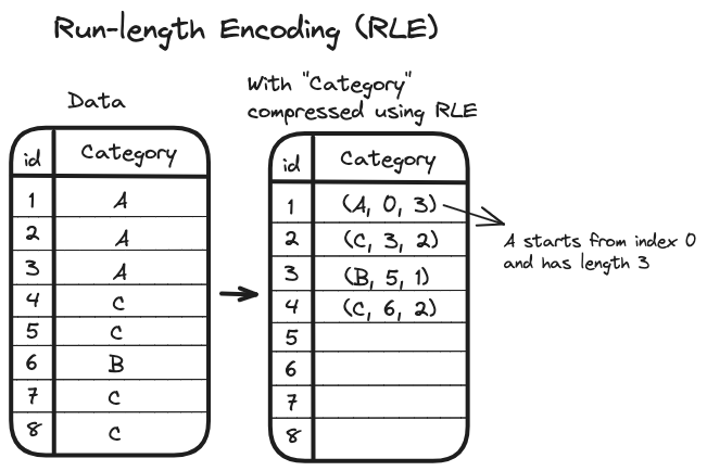
Run Length Encoding (RLE) is a compression technique that works by identifying "runs" in a bitmap. A run is a sequence of consecutive bits that are either all zeros or all ones. Once these runs are identified, we encode each run by pairing the bit value (which could be a single bit indicating 0 or 1) with the run’s length. For example,

But how do we go about encoding and decoding these values? Let’s start with encoding. The approach depends on the data. For cases with predictable run length or where the maximum length of a run is known to be limited, we can use a fixed length encoding. Let us see an example,

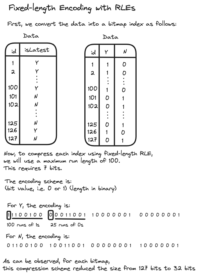
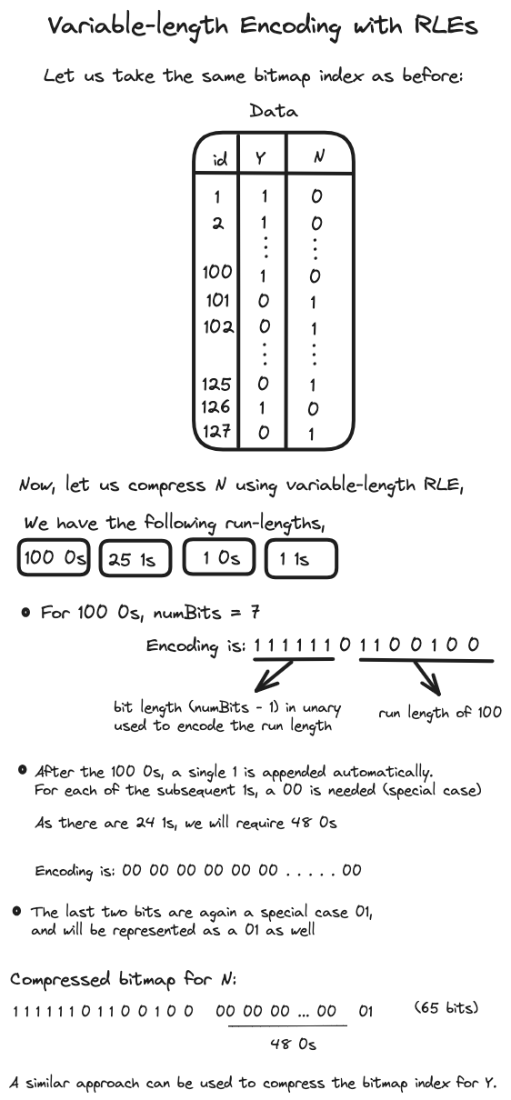
However, finding such constraints on run length can prove to be a challenge. As one might guess, allocating too few bits restricts the maximum run length that can be encoded, whereas allocating too many bits can reduce the compression efficiency for shorter runs. This is where the utility of a variable length encoding scheme becomes apparent.

Let's play around with this thought for a moment. How do we develop a variable length encoding scheme? Imagine we have a bitmap like 01000101, featuring three runs with lengths of 1, 3, and 1, respectively. A strategy for encoding could involve converting these runs into their binary representations and then concatenating them. For example, the binary equivalents of 1 and 3 are 1 and 11, respectively, leading to an encoding of 1111. However, a significant challenge with this approach is its lack of distinctiveness. For instance, a bitmap such as 00010101 would produce an identical encoded representation.

This underscores the need to differentiate the run length from the bit length used to encode said run length. Specifically, if there were a way to indicate that the encoding follows a pattern like {1}{111}{1}, with {} acting as delimiters, then we could readily address this issue.

And this is indeed how it is executed in practice. One particular scheme involves calculating the number of bits needed for the binary representation of a run length, which is approximately equal to \(log_2\\(\text{RL}\\)\). We denote this as \(numBits\), which is then expressed in unary notation by \(\\(numBits - 1\\)\) 1’s followed by a single 0. Following this, the binary representation of the run length is appended as before.

However, this approach presents two special cases. One occurs when encoding a sequence of “01”, and the other for a single “1”. For both scenarios, we assume \(numBits\) to be 1. The first case is addressed with a distinct encoding of “01”, and the second with “00”. Furthermore, using \(numBits - 1\) instead of \(numBits\) offers the advantage of saving one bit for non-special cases. Let us illustrate all of this with an example:

Figure 6: A step-by-step example for encoding bitmaps using variable-length RLE.

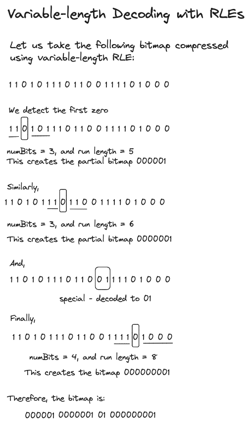
Decoding a bitmap is similar to the encoding process, where the detection of a zero prompts us to determine the run length indicated to its right, using the unary value to its left. Let’s demonstrate the decoding process with an example:

Figure 7: A step-by-step example for decoding bitmaps using variable-length RLE.

A notable drawback of RLE is that performing bitwise AND or OR operations on encoded bitmaps usually requires decoding them back to their original bitmap form. This situation is similar to that with Gzip and can lead to substantial overhead, particularly with frequent read operations in a database setting. While it is feasible to lazily perform this operation, it may still result in inefficiencies during random data access.

Byte-Aligned Bitmap Code

To address the decoding challenges associated with Run Length Encoding (RLE) and in the quest for a more efficient bitmap representation that inherently supports operations within them, Gennady Antoshenkov, then at Oracle, published a patent in 1994 for what is now known as Byte-Aligned Bitmap Code (BBC). As implied by its name, BBC operates on a byte-aligned basis, meaning it organizes bits into bytes without dividing bytes into individual bits during bitwise logical operations. This is important because processing whole bytes, as opposed to individual bits, is substantially more efficient on most CPUs, making byte-alignment critical to BBC's operational efficiency. While removing this alignment might yield better compression, it does so at the expense of slower bitwise operations.

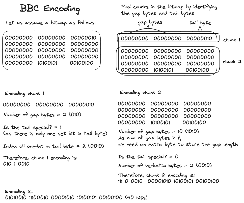
BBC codes fall into two categories: one-sided and two-sided codes. Let us first examine the one-sided codes. Each BBC is composed of two parts: a gap and a tail. The gap denotes the number of zero bytes preceding the tail. This tail may either be a single bit or a verbatim sequence of bitmap bytes. The choice of a single bit for the tail suits sparse bitmaps, whereas dense bitmaps necessitate verbatim byte sequences.

To encode and compress a bitmap with BBC, we divide the bitmap into "chunks". Each chunk is led by a header byte, succeeded by zero or more gap bytes, and then by zero or more tail bytes. The gap bytes are compressed via RLE, while the tail bytes are stored in their original form, except when considered special. A tail is special if it consists of only a single byte or contains just one non-zero bit.

The first three bits of the header byte indicate the length of the gap bytes. Should the gap byte length exceed six but stay below 128, an additional gap length byte is placed right after the header byte to capture the exact length. Similarly, if the length of the gap bytes is 128 or more but less than \(2^{15}\), then two gap length bytes are appended after the header byte. The fourth bit in the header byte indicates whether the tail is special or not. Furthermore, the header's final four bits specify the tail—either the number of tail bytes if the fourth header bit is 0, or they represent the non-zero bit's index within the tail byte if the fourth bit is 1.

Let's clarify this with an example of BBC encoding,

Two-sided codes are almost similar, with the distinction that the gap can be filled with either zeros or ones. This versatility is especially useful for encoding non-sparse bitmaps.

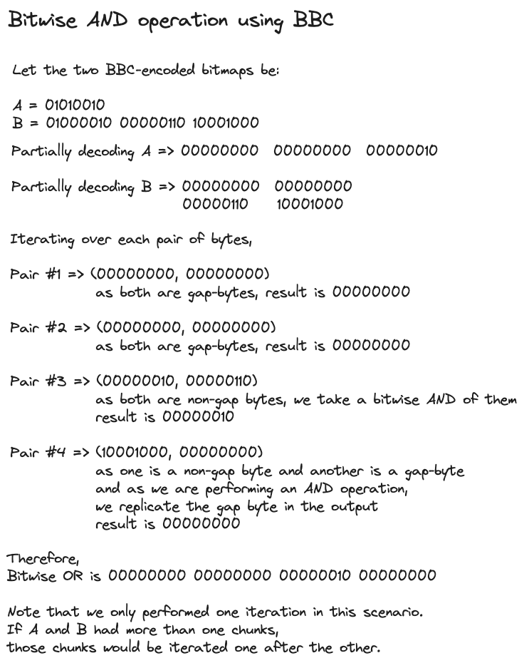
Now, to perform bitwise operations, let us consider two BBC-encoded bitmaps: one designated as the "left" bitmap and the other as the "right" bitmap. The process begins by partially decoding these bitmaps into corresponding left and right bytes. Next, we categorize each byte from the left and right as either a gap byte or a non-gap byte. If a byte pair is mismatched in category (i.e., one is a gap byte and the other is not), then for the AND operation, we bypass the non-gap byte and replicate the gap byte in the output. Conversely, for an OR operation, we overlook the gap byte and replicate the non-gap byte in the output. However, if both bytes are of the same type, we directly apply the intended bitwise operation (e.g., AND, OR) on these bytes to generate the merged output byte. This procedure is iterated until all byte pairs from the bitmaps have been merged.

This method shows the advantage over RLE, as it allows for the execution of bitwise operations using the tail bytes without necessitating an explicit decoding of those bits. An example of this is shown in the figure below:

Today, the BBC technique is largely considered outdated. Despite offering respectable compression, it is outperformed by more recent alternatives due to its tendency to induce excessive branching, a consequence of its header byte design. But what exactly is excessive branching, and why is it not optimal?

To understand this, we must first understand branch prediction. Branch prediction is an architectural feature that speeds up the execution of branch instructions (e.g., if-then-else statements) by trying to guess which way a branch will go before it is definitively known. A simple prediction method employs a 2-bit counter, where the states 00 and 01 indicate a prediction to "not take the branch," and the states 10 and 11 suggest to "take the branch," starting with an initial state of 10. Suppose we encounter a program counter, denoted as \(A\), which points to a branch instruction. If the prediction is to take the branch (as indicated by the state 10), but it is later determined that the branch should not have been taken, the prediction is adjusted by decrementing the counter by 1, i.e. to 01. This strategy proves useful when branches typically resolve consistently as either taken or not. However, the uncertainty introduced by the BBC header byte - such as the occasional presence or absence of an extra gap length byte - does not align well with CPU pipeline architectures. These branch statements, due to their unpredictable nature, cannot be efficiently anticipated through branch prediction, resulting in longer execution times.

Furthermore, BBC does not support random access of data within a bitmap. Due to these limitations, Oracle eventually transitioned to the Word-Aligned Hybrid code (WAH) to achieve better performance.

Word-Aligned Hybrid code

Before we discuss WAH, it is important to note that for many years, WAH was patented by the University of California. However, in November 2023, the patent expired as they seemed to have failed to pay the required maintenance fees.

WAH was introduced in 2010 by Kesheng Wu, Ekow J. Otoo, and Arie Shoshani, who were affiliated with the Lawrence Berkeley National Laboratory in California at the time. The goal of WAH was to offer a more CPU-friendly alternative to BBC by simplifying its header structure, thereby improving the execution speed. However, this was achieved at the cost of a less efficient compression ratio.

In contrast to BBC's byte alignment, WAH is - as its name implies - word-aligned. This means that it stores compressed data in words instead of bytes. A word represents the maximum amount of data that a CPU's internal data registers can hold and process at a time. Most modern CPUs today have a word size of 64 bits. Accessing a word typically takes as much time as accessing a byte. Therefore, by minimizing memory access frequency and optimizing memory bandwidth usage, a word-aligned approach proves significantly more efficient than a byte-aligned one.

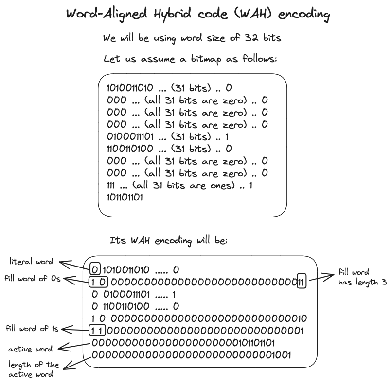
WAH distinguishes between two word types: literal words and fill words. Similar to the structure of BBC, a literal word directly represents a bitmap (a verbatim sequence of bytes), whereas fill words denote a fill of 0s or 1s. A word's most significant bit is used to differentiate a literal word from a fill word, with 0 indicating a literal word and 1 indicating a fill word. In the case of a literal word, the subsequent bits reflect the bitmap's bit values. For a fill word, the bits following the most significant one are split into two sections: the second most significant bit indicates the type of fill (either 0 or 1), and the remaining bits specify the fill's length.

Should the bitmap data not align perfectly with word groupings, the final word is labeled as an active word. It stores the last few bits that could not be grouped. This word is followed by another word, which specifies the count of useful bits in the active word.

Let's illustrate all of this with a figure:

For performing logical operations, we can apply the same algorithm used for BBC, but with WAH, each word is processed in an iteration instead of a byte.

To grasp the limitation of WAH, consider the following scenario:

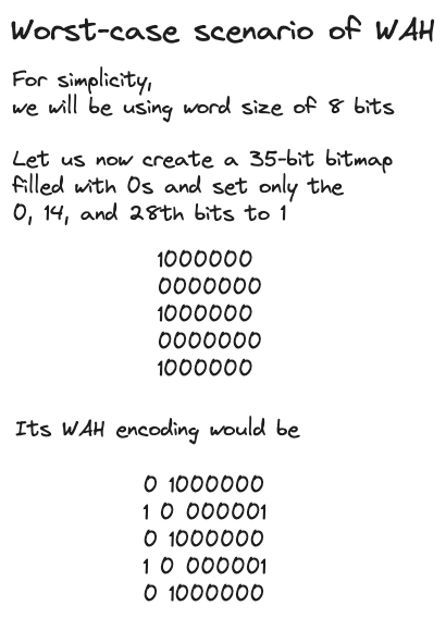
As evident, in such scenarios, WAH may require up to \(2w\) bits to represent a single set bit. These situations typically arise when there's a lengthy sequence of fill bits interrupted by one non-fill bit in the middle.

Concise

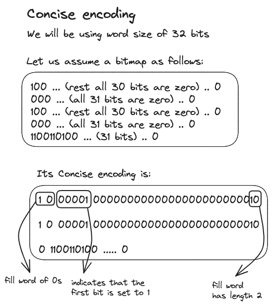
To address this shortcoming, Alessandro Colantonio and Roberto Di Pietro introduced a variation known as Compressed ’n’ Composable Integer Set (also known as Concise). It is similar to WAH with a notable distinction in the representation of the fill word. The fill word begins with its most significant bit set to 1, followed by a bit indicating the type of fill, yet the subsequent 5 bits are allocated to denote the position of a flipped bit within a long sequence of fills. For instance:

This adjustment helps mitigate the extreme cases observed earlier. While both methods show improved performance over BBC, they share a common limitation: their inability to perform random access. To overcome this, we will now turn our attention to the heart of this chapter - Roaring bitmaps.

Roaring Bitmaps

The main idea behind roaring bitmaps is to efficiently store 32-bit integers using a compact, two-level indexing structure. At the first level, the 32-bit index range is divided into "chunks" of \(2^{16}\) integers, each sharing the same 16 most significant bits. To store the 16 least significant bits, specialized “containers” are used.

Each chunk is categorized as either dense or sparse based on its content. A chunk is considered sparse if it contains 4096 integers or fewer, utilizing a sorted array of packed 16-bit integers for storage. Conversely, a chunk with more than 4096 integers is deemed dense and is represented using a \(2^{16}\)-bit bitmap. Here is an example of this encoding scheme:

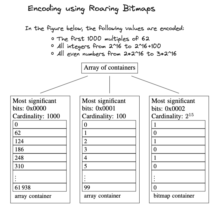
These containers are organized in a dynamic array, where the shared 16 most-significant bits act as a first-level index, ensuring the containers are sorted in order according to these bits. We will later see how sorting helps improve the speed of both random access and bitwise operations. The design of the first-level index ensures efficiency; for instance, indexing up to a million elements (binary representation: 11110100001001000000, containing 20 bits) requires at most 16 entries, allowing the structure to often remain within the CPU cache. Additionally, the container-level threshold of 4096 guarantees that no container exceeds 8 kB (\(2^{16}\) bits) in data representation.

Furthermore, each container tracks its own cardinality using a counter. This helps in quickly calculating the roaring bitmap's overall cardinality by summing the cardinality of each container.

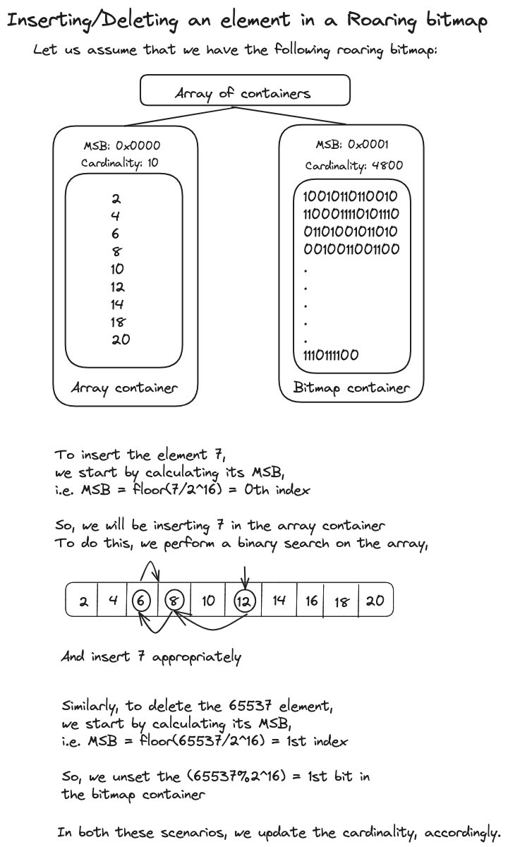
Having discussed this, let's now explore how this structure enables random access of data. To determine the presence of a 32-bit integer \(x\), we initially locate its position in the sorted first-level index using the 16 most significant bits of \(x\), i.e. \(\lfloor x/2^{16} \rfloor\). This can be done using a binary search. With this step, we gain access to the corresponding container. We then assess whether it is a bitmap container or a sorted array-based container. In the case of a bitmap container, we check the \((x\; \text{mod}\; 2^{16})^{\text{th}}\) bit (essentially, the index derived from the 16 least significant bits). For a sorted-array container, binary search is used once more, utilizing the value represented by the 16 least significant bits.

The same logic applies when inserting or removing an integer \(x\). The initial step involves locating the appropriate container. If the container is a bitmap, we adjust the relevant bit's value and update the cardinality as needed. Conversely, if an array container is encountered, we execute a binary search followed by a linear-time insertion or deletion. Here's how this operation work in practice:

And finally, we dive into bitwise operations on roaring bitmaps. A bitwise operation between two roaring bitmaps involves iterating through and comparing the 16 most significant integers (keys) in the sorted first-level index. This results in the creation of a combined roaring bitmap. During each iteration, if two keys match, a logical operation is performed between their respective containers, resulting in a new container. When the keys differ, the iteration advances the smaller key by one position. In an OR operation, the lower key and its corresponding container are included in the combined roaring bitmap.

OR operations continue until both sorted first-level arrays are exhausted, whereas AND operations terminate when either array exhausts out.

This logic naturally leads to the question: how do we execute a logical operation between specific containers? We encounter three scenarios here: operations between two bitmaps, a bitmap and an array, and two arrays.

In the case of two bitmaps, for an OR operation, we can directly compute the OR for each container pair. This approach is feasible because the cardinality of the resulting bitmap will always be at least as large as that of the original bitmaps, eliminating the need to create a new array container. The AND operation, however, requires a different approach. For AND, we first determine the cardinality of the result. If it exceeds 4096, we proceed as in the OR operation with a resulting bitmap. If the cardinality is below this threshold, we create a new array container and populate it with the set bits from the bitwise AND operations.

Keep in mind that while performing these operations, we consistently generate and update the new cardinalities of the combined roaring bitmap. At first glance, computing bitwise operations and their resultant cardinalities might seem like a slow process. However, the developers of roaring bitmaps have implemented several optimizations to address this concern. For example, processors from Intel, AMD, and ARM come equipped with instructions capable of quickly calculating the number of ones in a word. Intel and AMD provide a popcnt instruction (population count) that can perform this task with a throughput as high as operation per CPU cycle. Additionally, most modern processors are superscalar, meaning they can execute multiple instructions simultaneously. Therefore, as we process the next data elements, perform their bitwise operations, and store the results, the processor can concurrently apply the popcnt instruction to the previous result and increment the cardinality counter accordingly.

Tangentially, an interesting anecdote on the population count instruction is seen in Henry S. Warren, Jr.’s "Hacker’s Delight":

According to computer folklore, the population count function is important to the National Security Agency. No one (outside of NSA) seems to know just what they use it for, but it may be in cryptography work or in searching huge amounts of material.

The process for handling bitwise operations between a bitmap and an array is straightforward. During an AND operation, we iterate through the sorted dynamic array, and check for the presence of each 16-bit integer within the bitmap container, with the result being written into another dynamic array container. For OR operations, we duplicate the bitmap and iterate through the array, setting the appropriate bits.

Lastly, we come to the scenario involving two arrays. For an AND operation, we can use a simple merge algorithm, similar to that observed in merge sort.

In an OR operation, much like with two bitmaps, we must consider whether the cardinalities are above or below 4096. We begin by determining the resultant cardinality. If it does not exceed 4096, we merge the two dynamic arrays into one container using a merge algorithm. If the cardinality is higher, we set the bits for both arrays in a bitmap container, then assess the cardinality with popcnt. Should the cardinality not exceed 4096, we convert the bitmap container into an array container.

To illustrate a scenario where a bitmap container needs to be converted into an array container, consider container A with 4090 elements and container B with 10 elements. However, all 10 elements in B are already present in A. In this case, the resultant cardinality would be 4090, necessitating the conversion of the bitmap container back to an array container.

Another Roaring bitmaps paper introduces several other fascinating optimizations for this compression scheme. For example, in this subsequent work, they show how a third type of container, known as the run container, can efficiently store sequences of contiguous values (like all values from 1 to 100). We leave it to the curious reader to explore these ideas further.

←