Timing Wheels
The Secret World of Data Structures and Algorithms, Chapter 5
Author: Parth Parikh
First Published: 26/10/25
Come what come may, time and the hour runs through the roughest day.
- William Shakespeare, Macbeth
Welcome again to the draft of the fifth chapter of "The Secret World of Data Structures and Algorithms". It's been a while! The first four chapters can be checked out here. As always, I'm looking forward to your feedback.
In this chapter, we will start by discussing the evolution of timekeeping, leading all the way to its use in computers. We will then introduce software timer modules, and explain timing wheels as a fast and memory efficient way to manage timers. Finally, we will discuss both the classic Linux timer wheel implementation and its modern variant.
Hourglasses, Quartz, ENIAC, and Everything Between
There is something rather divine and powerful when discussing time. In this chapter, we will discuss a mechanism that mankind has used for eons to measure segments of time, which we call timers. Today, the word 'timer' is synonymous with a type of clock that starts from a specified duration and stops upon reaching zero. While this definition has literally stood the test of time, one might argue that the very embodiment of a clock has undergone quite a metamorphosis.
Perhaps the most iconic timer of all is the hourglass, first depicted in Ambrogio Lorenzetti's mural "The Allegory of Good and Bad Government", where Lady Temperance (a cardinal virtue) is seen holding an hourglass, symbolizing moderation. In the late Middle Ages and the Renaissance period, hourglasses were used in various settings - from ensuring that prayers were performed periodically in religious settings to regulating work shifts and cooking activities. Another fascinating use of hourglasses was in maritime navigation; they are accurate enough and not easily affected by the motion of the ship, no matter how violently the ship rocked. One interesting story about this is described by Laurence Bergreen in his book, "Over the Edge of the World: Magellan's Terrifying Circumnavigation of the Globe":
The privileged pages maintained the sixteen Venetian sand clocks—or ampolletas—carried by Magellan’s ships. Basically a large hourglass, the sand clock had been in use since Egyptian times; it was essential for both timekeeping and for navigation. The ampolletas consisted of a glass vessel divided into two compartments. The upper chamber contained a quantity of sand trickling into the lower over a precisely measured period of time, usually a half hour or an hour. Maintaining the ampolletas was simple enough—the pages turned them over every half hour, night and day—but the task was critical. Aboard a swaying ship, the ampolletas were the only reliable timepiece, and the captain depended on them for dead reckoning and changing the watches. A ship without a functioning ampolleta was effectively disabled.
The hourglass itself represents an upgraded form of the clepsydra or water clocks, which are some of the oldest time-measuring instruments. These timers used a container marked with lines, initially filled with water that would then slowly and evenly drain out. Such water clocks are governed by Torricelli's Law, named after Evangelista Torricelli's work four centuries ago on the effects of draining a tank through an opening. The law states that assuming an inviscid fluid (i.e., a fluid without viscosity), the efflux velocity (i.e., the speed at which the fluid exits an opening) equals the velocity that the fluid would acquire if allowed to fall from the free surface of the reservoir to the opening.
Clepsydra too has a rich set of tales to tell. It was possibly one of the earliest forms of stop watch. In the Athenian law courts it was used to allocate time to speakers. For civil suits and settlements, less water was used. However, when the topic revolved around serious political charges, more extensive water usage was allocated. J.G. Landels describes this in his paper on "Water-clocks and time measurement in Classical Antiquity":
The main purpose for which this type of klepsydra was used, curiously enough, was in law-court procedure. Greek orators, like their successors in most ages since, tended to be long-winded; in order to restrict them, and to ensure fairness to each side of the case, the klepsydra was used to time each speaker, and when it ‘ran out’ he was obliged to stop. The length of time depended on the nature of the case, and was measured in choes, the chous being a liquid measure corresponding to about 5.76 pints or 3.27 litres.
Interestingly,
The physician Herophilos, who worked in Alexandria in the early 3rd century BC, was very interested in the pulse, and in the significance of an increase in the pulse-rate (pyknosphyxiu, as he called it) as symptomatic of disorders. We are told that he had a small klepsydra which he took with him on visits to sick patients. He had worked out by empirical tests the normal number of heartbeats for persons of various age groups which ought to occur during the time measured by his klepsydra, and on arrival at the patient’s bedside he ‘placed down the klepsydra (i.e. set it going) and grasped the patient; and the amount by which the pulse-beats exceeded the normal number for that age-group was an indication of the mildness or intensity of the disorder.
As we know, these devices are largely antiquated today, having been replaced first by mechanical timers and now by timers using quartz clocks. Quartz clocks themselves have a fascinating history. In 1880, the then twenty-one-year-old Pierre Curie, along with his brother Jacques, discovered an unusual phenomenon in various crystals: when these crystals are stressed, an electric potential is induced in nearby conductors and, conversely, when such crystals are placed in an electric field, they deform slightly, in a manner proportional to the strength and polarity of that field. We today recognize this as the piezoelectric effect. In their 1880 paper, they experimented with tourmaline, topaz, quartz, calamine, and boracite, and had the following to say about quartz (translated into English):
In quartz, the two faces on which pressure is exerted must naturally be cut parallel to the main axis, and perpendicular to one of the three horizontal hemihedral axes, which our dear master, Mr. Friedel, recently demonstrated to be pyroelectric axes. The intensity of the phenomenon is quite notable in these three directions.
This discovery set the stage for quartz clocks, but it was not the only one. You see, before quartz clocks, mechanical clocks were the standard; however, they were significantly affected by factors such as mechanical wear and temperature, leading to decreased accuracy over time. A solution involved maintaining a precise and robust frequency, which was addressed by using an electrical oscillator to sustain the motion of a tuning fork. Later on, this approach was significantly improved with the discovery of quartz crystal oscillators, as mentioned in Shaul Katzir's paper:
… one of these researchers, Walter Cady, an American physics professor, turned his attention to an open-ended, and in this sense scientific, study of vibrating piezoelectric crystals unrelated to their use for submarine detection. He soon discovered that when quartz crystals vibrated at their “resonance frequency” (the frequency at which they provide the lowest resistance to vibration) their electrical properties changed sharply. Moreover, he observed that the crystals kept a highly stable resonance frequency. These natural properties of the crystals suggested to Cady that quartz crystals embedded in electronic circuits could be used as frequency standards for the radio range.
These discoveries eventually led to the construction of the first quartz clock in October 1927 by Joseph W. Horton and Warren A. Marrison, who were then at Bell Labs. The fascinating account of this discovery, along with its surrounding developments, is recounted by Warren Marrison himself in a 1948 paper titled 'The Evolution of the Quartz Crystal Clock'. Modern quartz watches today are built on these foundations, and one of their workings is concisely explained by Jonathan D. Betts in the Encyclopedia Britannica:
The timekeeping element of a quartz clock consists of a ring of quartz about 2.5 inches (63.5 mm) in diameter, suspended by threads and enclosed in a heat-insulated chamber. Electrodes are attached to the surfaces of the ring and connected to an electrical circuit in such a manner as to sustain oscillations. Since the frequency of vibration, 100,000-hertz, is too high for convenient time measurement, it is reduced by a process known as frequency division or demultiplication and applied to a synchronous motor connected to a clock dial through mechanical gearing. If a 100,000 hertz frequency, for example, is subjected to a combined electrical and mechanical gearing reduction of 6,000,000 to 1, then the second hand of the synchronous clock will make exactly one rotation in 60 seconds. The vibrations are so regular that the maximum error of an observatory quartz-crystal clock is only a few ten-thousandths of a second per day, equivalent to an error of one second every 10 years.
Eventually, this progress trickled its way down to computers. The background of timer modules in computers is equally rich. The first programmable general-purpose digital computer, completed in 1945 and known as the Electronic Numerical Integrator and Computer (ENIAC), featured dedicated timers in its 'initiating unit.' This unit was responsible for turning the power on and off, starting a computation, and performing initial clearing. Among other features, it included an adjustable timer set for 1 minute to provide for the delay between the turning on of the power supply heaters and plates, both components of vacuum tubes. The heaters warmed the vacuum tubes' cathodes to emit electrons, while the plates collected these electrons to control electronic signals. Once the timer reached the specified period (e.g., 1 minute), a relay—an electrically operated switch—would activate, connecting the plates of the power supplies to the AC control circuits so that the DC circuit could be turned on. Essentially, these timers managed the timing of the switch from AC to DC, used by ENIAC's electronic components, to help ensure that power was supplied in a controlled and sequential manner, preventing damage. A few years later, EDVAC also introduced a dedicated timer module to maintain synchronism throughout the machine.
Fast forward to today, virtually all computers have timer modules at both hardware and software levels. These usually rely on precisely machined quartz crystals, using a technique similar to the one mentioned above. Maarten van Steen and Andrew Tanenbaum have discussed this further in their book on Distributed Systems:
Associated with each crystal are two registers, a counter and a holding register. Each oscillation of the crystal decrements the counter by one. When the counter gets to zero, an interrupt is generated and the counter is reloaded from the holding register. In this way, it is possible to program a timer to generate an interrupt 60 times a second, or at any other desired frequency.
Timer Modules
In this chapter, we will focus our attention on software timer modules, particularly exploring a data structure known as 'Timing Wheels' which is used to efficiently manage timer events over a specified period.
At its core, a software timer module provides the necessary abstractions for programs to manage timers. They use the system's clock to track time and allow tasks to be scheduled and executed after a specified time interval. In an operating systems setting, timers are essential in constructing algorithms where the notion of time is critical. For instance, one way to schedule tasks is by using a technique called preemptive multitasking. Imagine a process running for a fixed amount of time before the operating system interrupts it and schedules another process. This new process again runs for a fixed time before it is interrupted, and this cycle continues. To do this, schedulers leverage a timer to periodically interrupt the CPU. While there is a context-switching overhead and managing concurrency can get tricky, such schedulers are quite useful in both single and multi-core systems, especially for real-time processing.
Another application of software timers is in controlling packet lifetimes for computer networks. For instance, a DNS (Domain Name System) resource record, along with the name of the domain, its type, and value, also stores a time to live (TTL) value. This helps determine the time a record is set to exist in the system before it can be discarded or revalidated. Indirectly, it gives an indication of how stable the DNS record is. A highly stable record might have values such as 86400 (the number of seconds in a day), whereas a volatile record might have a considerably small value.
Yet another use case for timers involves failure recovery. Consider, for instance, watchdog timers, which are widely used in embedded systems. Most embedded systems need to be self-reliant. Imagine remote systems such as space rovers, like the Mars Exploration Rover, which are not physically accessible to human operators. What happens when software hangs in such systems? A physical reboot is out of the question, and without a solution, these systems could become permanently disabled. To manage such cases, a watchdog timer is employed. It is a hardware timer used to automatically detect software anomalies and reset the processor if any occur. A counter is started with an initial value and is periodically decremented by 1. If it reaches zero at any point, the processor is restarted as if a human operator had cycled the power. To ensure this does not interfere with normal processing, the counter is reset back to its initial value after a periodic time interval to prevent it from "timing out." Tangentially, the reasoning behind the term "watchdog" is to draw a metaphor comparing the activity of resetting the counter the following:
The appropriate visual metaphor is that of a man being attacked by a vicious dog. If he keeps kicking the dog, it can’t ever bite him. But he must keep kicking the dog at regular intervals to avoid a bite. Similarly, the software must restart the watchdog timer at a regular rate, or risk being restarted.
Now, consider a scenario where the timer algorithms are implemented by a processor that is interrupted each time a hardware clock ticks, and the interval between ticks is on the order of microseconds. In such cases, the interrupt overhead can be substantial. Consider another scenario where very fine-grained timers are required to implement timer algorithms, and a large number of active timers need to be managed for some processes. In all these cases, managing the performance of timer modules is absolutely critical; otherwise, it can have a severe impact on runtime latency.
Such scenarios are becoming exceedingly common with the advent of cloud computing. Take the case of load balancers that check the health of servers at very short intervals. These systems regularly ping the underlying instances to ensure they are responding properly. This is important to avoid sending traffic to failed nodes. Similarly, cloud providers periodically check the load of servers using various metrics, such as CPU usage, memory consumption, and network traffic, to automatically scale resources — a process known as autoscaling. Towards the end of this chapter, we will explore some of these scenarios in greater detail. But before we explore this, let us understand the components of a timer module, how different timer schemes look like, and what their tradeoffs are.
We can conceptually divide a software timer module into four routines: start timer, stop timer, per tick bookkeeping, and expiry processing. The start timer routine starts a timer (associated with an id) that will expire after a specified interval of time. Once it expires, an expiry processing routine can be performed, such as calling a client-specified routine or setting an event flag. Moreover, the stop timer routine uses this id to locate a particular timer and stop it.
The per tick bookkeeping routine depends on the granularity of the timer, that is, how precisely we can measure time intervals using our timer module. A smaller granularity would help measure shorter and more precise intervals. If we measure our granularity in \(T\) units, then every \(T\) units, the per tick bookkeeping will check if any outstanding timers have expired. If they have, the stop timer routine will be invoked for each one of them.
In the most naive sense, a timer scheme can be implemented by maintaining a map between the timer identifier and its timer interval. Assuming that the per tick bookkeeping routine has a granularity of T units, then every T units, this scheme iterates over each timer interval and decrements them by T units. If at any time, an interval becomes zero, the timer identifier is used to stop the timer routine and start the corresponding expiry processing routine.
This scheme works fine when there are only a few outstanding timers and when the timers are stopped within a few ticks of the clock. For most other cases, the bookkeeping routine can be quite expensive and might require special-purpose hardware.
A natural iteration of this approach is to store timers in an ordered list (also known as timer queues). In this scheme, instead of storing the time interval, an absolute timestamp is stored. The timer identifier and its corresponding timestamp that expires the earliest is stored at the head of the queue. Similarly, the second earliest timer is stored after the earliest, and so on, in ascending order. After every \( T\) unit, only the head of the queue is compared with the current timestamp. If the timer has expired, we dequeue the list and compare the next element. We repeat this until all the expired timers have been dequeued, and we run their expiry processing routines.
In this scenario, the per tick bookkeeping is only required to increment the current timestamp by \(T\) units, rather than decrementing each individual timer intervals by \(T\) units. However, the worst-case latency to start a timer can be \(O(n)\), which is observed when all the timers in the queue expire during the same granularity interval of \(T\) units. This would require all of the timers to be dequeued before the first one can start its expiry processing routine. As you can imagine, the average latency would therefore be dependent on the distribution of arrival time of the timers and their relative timer intervals.
Interestingly, we can employ a theorem from Queuing Theory known as Little's Law to determine the average number of timers in the queue. It says that the average number of items in a queuing system, denoted \(L\), equals the average arrival rate of items to the system, \(\lambda\), multiplied by the average waiting time of an item in the system, \(W\). Thus, \(L = \lambda W \). So, if there are 3 timers per minute (\(\lambda\)) and a timer interval is on average 5 minutes \((W)\), then the average number of timers in the queue \((L)\) would be 15.
If a dynamic array is used to store this ordered list, the latency of insertion is \(O(n)\). This is because finding the correct position of insertion can take \(O(\text{log}\;n)\) using binary search. Further, once the insertion position is found, shifting all the subsequent timers after this position to the right can be at most \(O(n)\). This can be considerably improved by using a balanced binary search tree or binary heaps.
Timing Wheels
Having explored this, we can now dive into the soul of this chapter — Timing Wheels, which is yet another way to implement timer algorithms. To understand the motivation behind Timing Wheels, it's worth asking ourselves what one of the fastest theoretical timer algorithms would look like. One way to implement this would be by constructing a linear array of lists (also known as timer buckets), where each index (or timer bucket) represents a timer interval \( T \) that corresponds to a single clock tick, and a running index pointer \( \text{IP} \) keeps track of the current timer interval position. Such an array could start at a timer interval of \(0\) and end at some maximum interval value (\(\text{maxInterval}\)). The number of timer buckets that can be accommodated, denoted as \( N \), would be \( N = \lceil \text{maxInterval} / T \rceil \).
To add a timer \( j \) units past its current timestamp, we push it into the list in the timer bucket at the index \(\left(\text{IP} + j\right) \bmod N\).
Given an index position and a timer ID, stopping the timer is as simple as searching for the specified ID in the list maintained by the corresponding timer bucket and removing the timer from that list. Subsequently, expiring the timer involves advancing the \(\text{IP}\) by one and expiring all (if any) timers in the next timer bucket. This way, adding, stopping, and expiring a timer all have a constant \( O(1) \) overhead on average.
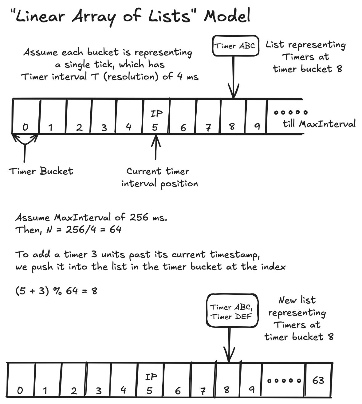
While it looks good in theory, such a concept becomes nearly impossible to maintain in practice due to its huge memory footprint. For instance, to implement 32-bit timers, where every value is associated with a timer interval, one might require approximately \(2^{32}\) words of memory. To improve upon this, it becomes necessary to trade some computational cost for a reduced memory footprint.
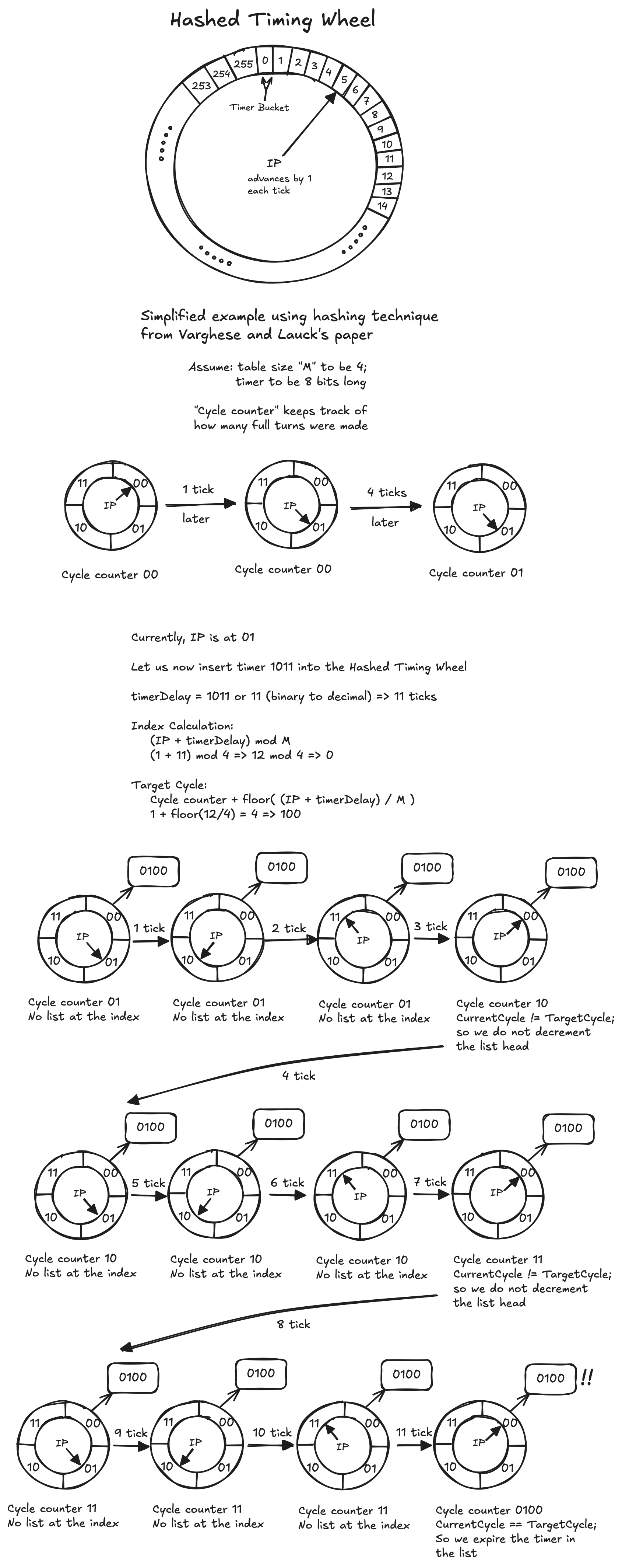
This is where hashed wheels come into play. To address insufficient memory, we can hash the timer expiration time (or timer delay) to yield an index. For example, one way to achieve this is by assuming the table size to be a power of 2. In such scenarios, an arbitrarily sized timer expiration time (labeled as \(\text{timerDelay}\)) can easily be divided by the table size \(M\). The index within the array is computed as \( \text{index} = (\text{IP} + \text{timerDelay}) \bmod M \). The number of full wheel revolutions to wait is \( \text{rounds} = \bigl\lfloor (\text{IP} + \text{timerDelay})/M \bigr\rfloor \), and we store with the timer an absolute \( \text{targetCycle} = \text{currentCycle} + \text{rounds} \) (so per tick we compare, not subtract).
As an illustration, consider the table size to be \(2^8\) (so \(M=256\)) and the timer to be 32 bits long. Then, the remainder from the division is the last 8 bits (\(\text{timerDelay} \bmod 256\)). If \(\text{timerDelay}\) is 120 ticks and the current \(\text{IP}\) is at 30, the index within the array would be \((30 + 120) \bmod 256 = 150\). We then place the timer in the list pointed to by the \(150^{\text{th}}\) index, storing \( \text{targetCycle} = \text{currentCycle} + \text{rounds} \). In this scenario, the wheel revolutions to wait is \( \text{rounds} = \bigl\lfloor (30 + 120)/256 \bigr\rfloor = 0 \), and \( \text{targetCycle} = \text{currentCycle} \). Equivalently, you can think of it as triggering this timer at the index \(150^{\text{th}}\) after 120 ticks. If the \(\text{targetCycle}\) were 1 instead, we would be triggering it off in the next cycle.
There are two ways to maintain a list for hashed wheels: keep a sorted list or an unsorted list. With a sorted list, the start timer can be slow as the higher order bits (effectively \(\text{rounds}/\text{targetCycle}\)) must be inserted into the correct place in the list. This is \(O(n)\) in the worst case, however, as before, it can be considerably improved by using a balanced binary search tree or binary heaps. Furthermore, as mentioned in Varghese and Lauck's paper, in practice the start timer cost is much better:
the average latency can be \(O(1)\). This is true if \(n \lt \text{TableSize}\), and if the hash function \(\text{Timer Value}\mod \text{TableSize}\) distributes timer values uniformly across the table. If so, the average size of the list that the \(i^{th}\) element is inserted into is \(i - 1/\text{TableSize}\). Since \(i \lt n \lt \text{TableSize}\), the average latency of StartTimer is \(O(1)\). How well this hash actually distributes depends on the arrival distribution of timers to this module, and the distribution of timer intervals.
The per tick bookkeeping routine for hashed wheels works by incrementing the \(\text{IP}\) by one (mod \(M\)) to yield the next index. If the value stored in the array element being pointed to is empty, there is no expiry processing needed.
Else, we need to examine the list at that index. Using simple comparison, we can dequeue and expire all timers whose \( \text{currentCycle} == \text{targetCycle} \). Naturally, timers with \( \text{targetCycle} \gt \text{currentCycle} \) remain in place. This takes \(O(1)\) on average with an \(O(n)\) worst case complexity, with the latter being observed when all the timers are due to expire at the very same instant.
Linux's Classical Timer Wheel
Let us switch gears and discuss how the Linux kernel uses timing wheels. Flattening a few nuances, the kernel has two underlying timer engines: a low-resolution jiffy-based timer wheel and a high-resolution hrtimer.
As Gleixner and Niehaus point out, this distinction matters because it dabbles in the subtle difference between a timeout and a timer. Timeouts are primarily used to detect when an event does not occur as expected. Imagine the case of a TCP retransmission, a SCSI/NVMe request timeout, or watchdog timers from our earlier example, whereas timers are used to schedule ongoing events — for example, preempting tasks at precise time-slice boundaries.
The kernel documentation describes the applications of low and high resolution timers in greater detail:
….. the timer wheel code is most optimal for use cases which can be identified as “timeouts”. Such timeouts are usually set up to cover error conditions in various I/O paths, such as networking and block I/O. The vast majority of those timers never expire and are rarely recascaded because the expected correct event arrives in time so they can be removed from the timer wheel before any further processing of them becomes necessary. Thus the users of these timeouts can accept the granularity and precision tradeoffs of the timer wheel, and largely expect the timer subsystem to have near-zero overhead. Accurate timing for them is not a core purpose - in fact most of the timeout values used are ad-hoc. For them it is at most a necessary evil to guarantee the processing of actual timeout completions (because most of the timeouts are deleted before completion), which should thus be as cheap and unintrusive as possible.
….. the primary users of precision timers are user-space applications that utilize nanosleep, posix-timers and itimer interfaces. Also, in-kernel users like drivers and subsystems which require precise timed events (e.g. multimedia) can benefit from the availability of a separate high-resolution timer subsystem as well.
In this chapter, we will be focusing on low-resolution timer wheels. We will start by looking into the design that existed during the 2.6 kernel update and iterate upon it by exploring the newer developments brought about by the 4.6 kernel update.
We begin with the question — what is a jiffy? To help define timer interrupts, the kernel uses a unit called a jiffy. This is defined as the time between two successive clock ticks. Therefore, its plural, "jiffies", holds the number of clock ticks that have occurred since the system booted.
The kernel keeps track of these jiffies using a global variable
initialized in the
jiffies.h file. In fact, you can take a peek at your system's jiffies using the
cat /proc/timer_list | grep "jiffies:" command. To find out
what 1 jiffy corresponds to in milliseconds on your system, you can run
"grep CONFIG_HZ /boot/config-$(uname -r)". The
CONFIG_HZ parameter
determines the timer interrupt frequency. By dividing it by 1, we get
the jiffy duration in milliseconds. For instance, my system has a timer
interrupt frequency of 250 Hz, and therefore the jiffy duration is 0.004
s or 4 ms.
This brings up a rather fascinating question — with a 4 ms jiffy, what
is the longest delay we can set for a timer? Well, it depends. In the
Linux kernel, the maximum such delay we can ask for is capped by the
MAX_JIFFY_OFFSET macro, as seen in the
jiffies.h file. For the
older 2.6 kernel on a 32-bit system, this used to be \( ((\sim0\text{UL} \gg 1) - 1) \), or \( (2^{32} \gg
1) - 1 \), which would correspond to \( 2147483647 \times 0.004 / 86400
\), or 99.42 days. However, today MAX_JIFFY_OFFSET is a signed long — \(
((\text{LONG_MAX} \gg 1) - 1) \). For 64-bit systems, the longest delay
would then be \( ((2^{63} \gg 1) - 1) * 0.004 / 86400 / 365 \), or
roughly \( 5.8 \times 10^8 \) years. Long enough to potentially cause a
mass extinction of all animal species, eh?
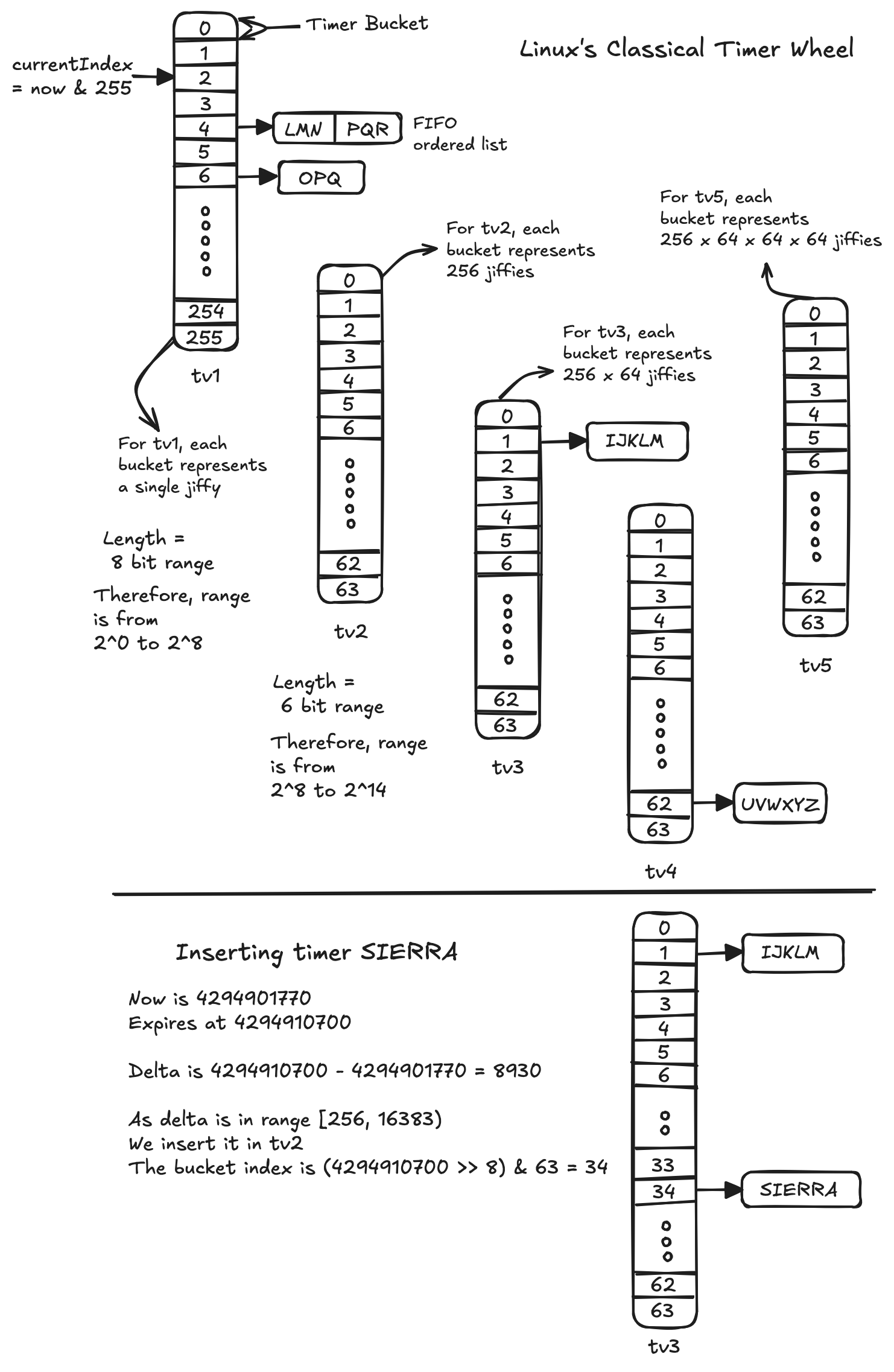
Let us now look into the design of the kernel's Timer Wheel itself. This architecture draws inspiration from the "linear array of lists" model that we have seen previously. Recall that, with such a model, each index corresponded to a timer bucket. Similarly, we could ideally represent each jiffy as a bucket; however, as before, that would blow up the memory footprint.
To prevent this, the kernel categorizes all future jiffies into a "logarithmic array of arrays" architecture. This involves dividing all future jiffies into 5 groups:
-
Group 1: Consists of 256 buckets, each representing a single jiffy.
- This group encompasses the range 0 to 255.
-
Group 2: 64 buckets, with each bucket representing 256 subsequent
jiffies.
- Range of 256 to 16,383.
-
Group 3: 64 buckets, with each bucket representing \( 256 \times 64
\), or 16,384 jiffies.
- Range of 16,384 to 1,048,575.
-
Group 4: 64 buckets, with each bucket representing \( 256 \times 64
\times 64 \), or 1,048,576 jiffies.
- Range of 1,048,576 to 67,108,863.
-
Group 5: 64 buckets, with each bucket representing \( 256 \times 64
\times 64 \times 64 \), or 67,108,864 jiffies.
- Range of 67,108,864 to 4,294,967,295.
Each group is represented using fixed-size arrays called the timer vectors: \( \text{tv1}, \text{tv2}, \text{tv3}, \text{tv4} \) and \( \text{tv5}\). Each index in a timer vector is associated with a linked list to represent multiple timers at the corresponding jiffy. With this, the kernel can split the 32 bits (4,294,967,296) of the timeout value into \( 8+6+6+6+6 \) bits. But how does this architecture perform insertion, deletion, and expiry processing?
Insertion is a constant time operation with at most 5 conditional statements. Consider "\(\text{expires}\)" to be the absolute jiffy when the timer should fire, and "\(\text{now}\)" to be the system's current jiffy. Using these, we can define "\(\text{delta}\)" as "\(\text{expires} - \text{now}\)". With this:
-
If \(\text{delta}\) is in the range \([0, 255)\)
- We insert it into \(\text{tv1}\).
- The bucket index is "\(\text{expires} \; \& \; 255\)".
-
Else if \(\text{delta}\) is in the range \([256, 16383)\)
- We insert it into \(\text{tv2}\).
- The bucket index is "\( (\text{expires} \gg 8) \; \& \; 63 \)".
-
Else if \(\text{delta}\) is in the range \([16384, 1048575)\)
- We insert it into \(\text{tv3}\).
- The bucket index is "\( (\text{expires} \gg (8 + 6)) \; \& \; 63 \)".
-
Else if \(\text{delta}\) is in the range \([1048576, 67108863)\)
- We insert it into \(\text{tv4}\).
- The bucket index is "\( (\text{expires} \gg (8 + 6 + 6)) \; \& \; 63 \)".
-
Else if \(\text{delta}\) is in the range \([67108864, 4294967295)\)
- We insert it into \(\text{tv5}\).
- The bucket index is "\( (\text{expires} \gg (8 + 6 + 6 + 6)) \; \& \; 63 \)".
Once we have the bucket index for a timer vector, we insert the timer at the back of a list at that index. Notice how the above insertion algorithm is an \(O(1)\)-time operation. This is natural since there are no loops in our bucket calculations — just a few comparisons, shifts, and masks.
When time advances, the "\( \text{now} \)" value gets incremented by 1. Subsequently, the new "\(\text{now} \; \& \; 255\)" position is treated as an index into \( \text{tv1} \). The list of timers at that bucket, if any, is first copied to a local work list and then their expiry processing routines are executed in a FIFO (First In, First Out) order.
To illustrate this with an example:
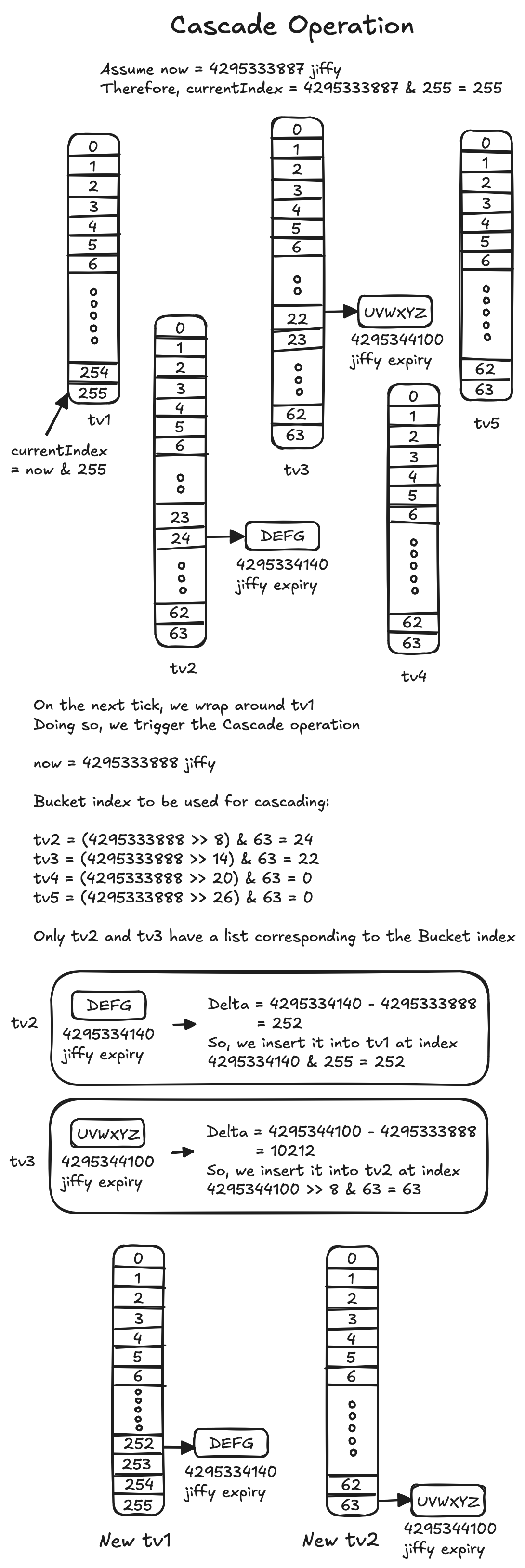
Intuitively, this insertion algorithm uses a timer's relative distance from "\( \text{now} \)" (labeled as "\( \text{delta} \)") to figure out the timer vector and its corresponding bucket it should be associated with. The near-term timers go straight into \( \text{tv1} \) (one slot per jiffy), while farther-out timers sit in coarser timer vectors (\(\text{tv2}\)-\(\text{tv5}\)). As time ticks, \(\text{tv1}\)'s "\(now \; \& \; 255\)" bucket index will eventually "wrap" around and reach 0 again. When that happens, the kernel performs an operation called Cascade.
Understanding the cascade operation is key to figuring out how expiry processing works for the timers sitting in the coarser timer vectors (\(\text{tv2}-\text{tv5}\)). The operation has two purposes:
- To move one bucket (or cascade it) from \(\text{tv2}\) to a lower level; if \(\text{tv2}\) wraps around and reaches 0 too, move a bucket from \(\text{tv3}\) to a lower level; if \(\text{tv3}\) wraps around and reaches 0 too, move a bucket from \(\text{tv4}\) to a lower level; and so on.
- Start the next lap of \(\text{tv1}\)
The cascade operation takes place as follows:
- Determine the bucket index to be used for cascading:
- \(\text{tv2}\) is \( (\text{now} \gg (8)) \; \& \; 63 \)
- \(\text{tv3}\) is \( (\text{now} \gg (8 + 6)) \; \& \; 63 \)
- \(\text{tv4}\) is \( (\text{now} \gg (8 + 6 + 6)) \; \& \; 63 \)
- \(\text{tv5}\) is \( (\text{now} \gg (8 + 6 + 6 + 6)) \; \& \; 63 \)
- Next, move the entire list at the bucket index to a temporary list \(\text{Tlist}\). Then, for each timer in \(\text{Tlist}\), call the insertion algorithm again. Use the timer's "\(\text{expires}\)" value to recompute the new "\(\text{delta}\)".
Notice how, in step 1, the shift and mask operations for determining the bucket index resemble the insertion algorithm, except that we use the "\( \text{now} \)" value instead of "\( \text{expires} \)". To demonstrate this operation:
Calculating the time complexity of the cascade operation may sound tricky at first glance. But try to visualize the following scenario: many timers bunch up in the same bucket, and we are about to hit jam-packed buckets for each of \(\text{tv2}\), \(\text{tv3}\), \(\text{tv4}\), and \(\text{tv5}\). On that "\(\text{wrap}\)", the cascade must re-enqueue every timer in those buckets. If those buckets together hold \(N\) timers (in the extreme, almost all pending timers), the processing time for that jiffy tick becomes \(O(N)\). However, as each timer is only cascaded a small, fixed number of times, the amortized cost of this operation is still \(O(1)\). In other words, the average per-timer cost stays constant.
The delete operation, by comparison, is rather simple. When we set a timer, the kernel keeps its address around. To delete a timer, it goes to that address and checks whether the timer is still waiting to fire. If yes, it unlinks that timer from whatever bucket list it's in (i.e., it removes that timer from the list and fixes up the neighbors) and returns 1. However, if the timer has already fired, it does nothing and simply returns 0. As with insertion, this operation is in \( O(1) \) time, too.
It is again worth stressing that the ability to immediately locate expired entries, insertion operations, and deletion operations are all constant-time. This makes it a perfect recipe for timeouts, which, as mentioned before, are the majority of timer-wheel use cases. These timers will usually be cancelled before they expire.
The Modern Wheel
While this implementation has aged over the past two decades, its foundations can still be seen in the kernel codebase. Today, however, the kernel's timer wheel has been refined based on the deficiencies of the older system.
For one, the
cascade operation
is done away with. What made it suboptimal was its unpredictability. As the amount of
work scales with how many timers happen to be in the higher-level
buckets, the cost can vary wildly. The kernel timers are expired in the
TIMER softirq (software interrupt requests) handler. If
many timers land in the same bucket that is about to be cascaded down,
the TIMER softirq can run for a long time. This, in turn,
can cause other softirqs such as NET_TX/RX (network packet
transmission and retransmission) and IRQ_POLL (used to poll
hardware devices) to sit queued, which ends up causing long softirq
latency. It is worth noting that the kernel does add an upper bound to
maintain fairness (see MAX_SOFTIRQ_TIME); nevertheless, bursts can still create latency.
The new timer wheel was architected around the realization that not all timers have to be handled with the same level of accuracy. Today's timer wheel is divided into 8 or 9 groups depending on the timer interrupt frequency. Every group has 64 buckets in it.
Just like before, each group is represented using an array of lists, with each array member reflecting a bucket of the timer wheel. The list contains all timers that are enqueued into a specific bucket. The lowest array (first group) contains timer events with one jiffy per bucket, as before. The array after that (second group) contains timer events with a resolution of eight jiffies per bucket. Similarly, the next group contains timer events with a resolution of 64 jiffies per bucket. And this trend goes on. Concisely, the granularity growth per group is consistently \( \times 8 \) of the group before. This can be shown as follows:
For groups \( n \ge 1 \),
The resolution of the bucket in group \( n \) is \( 8^n \) jiffies.
The range covered by group \( n \) is from \( 64 \times 8^{n-1} \) up to
\( 64 \times 8^n - 1 \) jiffies.
Here is one such example of the granularity and range levels mentioned in the modern kernel codebase:
* HZ  250
* Level Offset  Granularity            Range
*  0       0         4 ms                0 ms -        255 ms
*  1      64        32 ms              256 ms -       2047 ms (256ms - ~2s)
*  2     128       256 ms             2048 ms -      16383 ms (~2s - ~16s)
*  3     192      2048 ms (~2s)      16384 ms -     131071 ms (~16s - ~2m)
*  4     256     16384 ms (~16s)    131072 ms -    1048575 ms (~2m - ~17m)
*  5     320    131072 ms (~2m)    1048576 ms -    8388607 ms (~17m - ~2h)
*  6     384   1048576 ms (~17m)   8388608 ms -   67108863 ms (~2h - ~18h)
*  7     448   8388608 ms (~2h)   67108864 ms -  536870911 ms (~18h - ~6d)
*  8     512  67108864 ms (~18h) 536870912 ms - 4294967288 ms (~6d - ~49d)
As mentioned earlier, the modern kernel codebase has gotten rid of cascade operations in its entirety. This is perfectly summarized by Jonathan Corbet in LWN:
The old timer wheel would, each jiffy, run any expiring timers found in the appropriate entry in the highest-resolution array. It would then cascade entries downward if need be, spreading out the timer events among the higher-resolution entries of each lower-level array. The new code also runs the timers from the highest-resolution array in the same way, but the handling of the remaining arrays is different. Every eight jiffies, the appropriate entry in the second-level array will be checked, and any events found there will be expired. The same thing happens in the third level every 64 jiffies, in the fourth level every 512 jiffies, and so on. The end result is that the timer events in the higher-level arrays will be expired in place, rather than being cascaded downward. This approach, obviously, saves all the effort of performing the cascade.
As you can imagine, this comes with an accuracy tradeoff! Remember what I mentioned earlier: the new timer wheel was architected around a realization that not all timers have to be handled with the same level of accuracy — that is, the needs for timeouts differ from those of high-precision timers. With 64 buckets in the first group, anything more than 63 jiffies ahead no longer has single-jiffy accuracy; it has to be moved to the second group or higher. Now imagine a timeout that is 68 jiffies in the future. It will be placed in the next higher eight-jiffy slot — 72 jiffies in the future. With no cascades, this timer event will expire 4 jiffies later than requested. This effect naturally gets exacerbated as you move into the higher groups.
It is interesting to contrast all of this discussion with Linux's humble origins. Back in the days of yore, the kernel did not have to account for high-performance workloads, so they went for the simplest model: putting all the timers into a doubly-linked list and sorting the timers at insertion time. That model presented O(N) insertion time, \(O(N)\) removal time, and \(O(1)\) expiry processing time. As the saying goes, first we make it work, then we make it right, and finally we make it fast.
←