Approximate Distance Oracles
Author: Parth Parikh
First Published: 14/05/21
“One day Alice came to a fork in the road and saw a Cheshire cat in a tree.
- Lewis Carroll, Alice in Wonderland
‘Which road do I take?’ she asked.
‘Where do you want to go?’ was his response.
‘I don’t know,’ Alice answered.
‘Then,’ said the cat, ‘it doesn’t matter.”
Table of Contents
- Single-Source Shortest-Path Problem
- All-Pairs Shortest-Path Problem
- All-Pairs Approximate Shortest-Path Problem
- Approximate Distance Oracles
- (2k-1)-approximate distance oracles
- Conclusion
Note: To my knowledge, this is the first non-academic description of Approximate Distance Oracles. Furthermore, this is my first time writing about Graph Theory. Therefore, if you find any mistakes, please do let me know.
Summary: Approximate Distance Oracles can be used to approximately find out the distance between any two vertices in a graph. They help solve the all-pairs shortest path problem. This problem can also be solved using classical algorithms like Floyd-Warshall and Dijkstra's applied to n vertices. However, the difference here is that while classical algorithms provides you the exact distance, approximate distance oracles provides you an "approximation".
Single-Source Shortest-Path Problem
Let us assume that we have an undirected graph with strictly positive edge weights. Let us also assume that this graph represents the fictional city - The Ten Blocks. Here is an aerial view of this city -
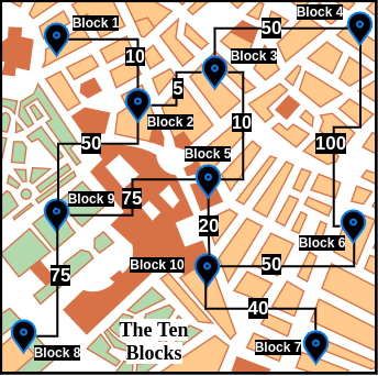
As The Ten Blocks' map can be cumbersome to visualize, for the rest of this blog post, we will be working with a simplified version -

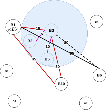
When we visualize this city as a graph, we notice that it has 10 vertices and 11 edges. Each vertex has a label of the form Block N, with N being any unique integer (for the rest of this blog post, we will abbreviate Block N as BN). The edge weight is the distance between two blocks. For example, the weight of the edge between B1 and B2 is 10. Furthermore, the length of a path between any two blocks is the sum of all the edge weights connecting that path. For example, the path (B1, B2, B3) has a length of 10+5=15. However, one should note that this is not the only path from B1 to B3. Another path is (B1, B2, B9, B5, B3) which has a path length of 10+50+75+10=145. Certainly a costly one!
A widely studied question about graphs is the shortest path problem, which is:
the problem of finding a path between two vertices (or nodes) in a graph such that the sum of the weights of its constituent edges is minimized.It can be observed visually that the shortest path between B1 and B3 is indeed (B1, B2, B3) with a path length of 10. But how do we algorithmically find the shortest paths between two vertices? One way is by using Dijkstra's algorithm. While a thorough analysis of Dijkstra's algorithm is beyond the scope of this blog post, the algorithm mentioned in the Wikipedia page on Dijkstra's algorithm is an excellent start -
Let the node at which we are starting be called the initial node. Let the distance of node Y be the distance from the initial node to Y. Dijkstra's algorithm will assign some initial distance values and will try to improve them step by step.
- Mark all nodes unvisited. Create a set of all the unvisited nodes called the unvisited set.
- Assign to every node a tentative distance value: set it to zero for our initial node and to infinity for all other nodes. Set the initial node as current.
- For the current node, consider all of its unvisited neighbours and calculate their tentative distances through the current node. Compare the newly calculated tentative distance to the current assigned value and assign the smaller one. For example, if the current node A is marked with a distance of 6, and the edge connecting it with a neighbour B has length 2, then the distance to B through A will be 6 + 2 = 8. If B was previously marked with a distance greater than 8 then change it to 8. Otherwise, the current value will be kept.
- When we are done considering all of the unvisited neighbours of the current node, mark the current node as visited and remove it from the unvisited set. A visited node will never be checked again.
- If the destination node has been marked visited (when planning a route between two specific nodes) or if the smallest tentative distance among the nodes in the unvisited set is infinity (when planning a complete traversal; occurs when there is no connection between the initial node and remaining unvisited nodes), then stop. The algorithm has finished.
- Otherwise, select the unvisited node that is marked with the smallest tentative distance, set it as the new "current node", and go back to step 3.
When planning a route, it is actually not necessary to wait until the destination node is "visited" as above: the algorithm can stop once the destination node has the smallest tentative distance among all "unvisited" nodes (and thus could be selected as the next "current").
To visualize the above Dijkstra's algorithm in practice, here is an example that uses The Ten Blocks graph -
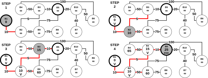
The working we described above is part of the single-pair shortest path problem. This is because, we were primarily interested in the shortest path between one pair (which in the above example was (B1, B5)). However, Dijkstra's algorithm can be used for a more general class of problems called single-source shortest path problems. This variant can be defined as:
A problem in which we have to find shortest paths from a source vertex v to all other vertices in the graph.Let us assume that in Figure 3, there was no endpoint. Instead, we want to find the shortest path from B1 to all the other 9 points. In this scenario, as per Dijkstra's algorithm mentioned above, we stop when we have visited (exactly once) every node in the graph (starting with B1). Here is a step-by-step process of the same -
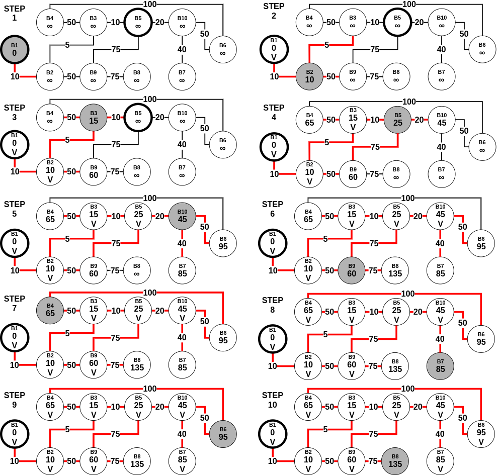
Assuming n is the number of vertices in the graph, Dijkstra's algorithm requires no more than (n-1) steps, with each step requiring no more than (n-1) comparisons to check if the vertex is not visited before, and no more than (n-1) comparisons to update the labels at each step. All in all, it uses O(n2) operations for additions and comparisons for the single-source shortest path problem.
All-Pairs Shortest-Path Problem
A natural succession to the single-source shortest path problem is the all-pairs shortest path problem (APSP), which is defined as:
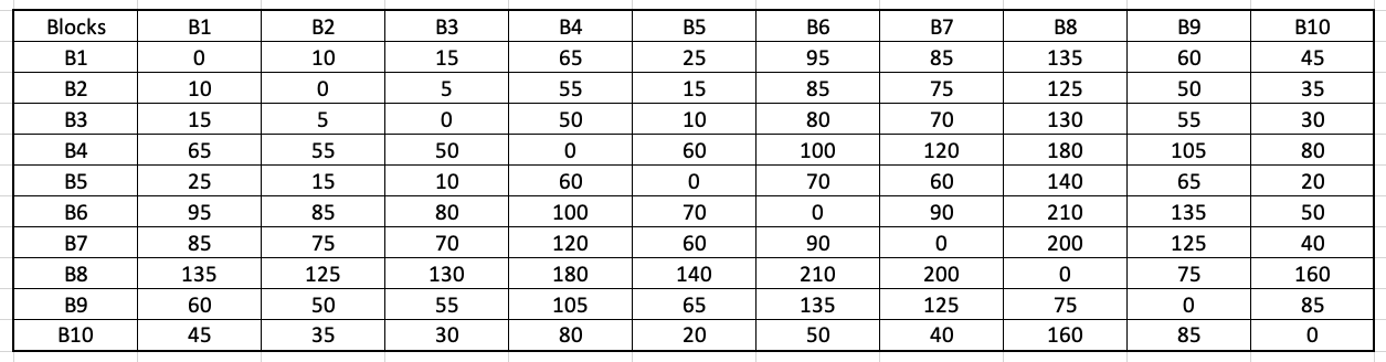
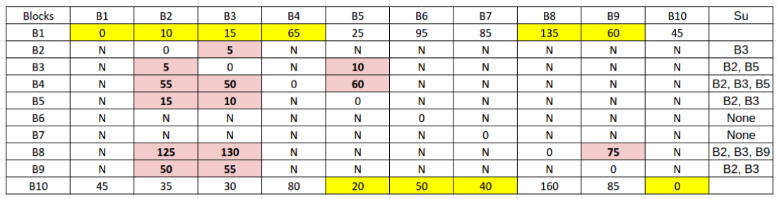
A problem in which we have to find the shortest paths between every pair of vertices v, v' in the graph.Keeping our previous assumptions valid (the graph is undirected and has positive edge weights), the easiest solution to the above problem would be to run Dijkstra's algorithm on every vertex in the graph. In doing so, we will obtain the following matrix:
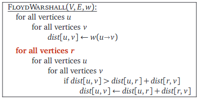
This algorithm is from the textbook Algorithms by Jeff Erickson (chapter 9). The book's contents are licensed under Creative Commons Attribution 4.0 International license.
Wikipedia contains a step-by-step example of the above algorithm. As can be observed, this algorithm has a time complexity of O(n3). At this point, a curious reader might be wondering - are the runtime between Floyd-Warshall and Dijkstra-based APSP the same? Here is what Prof. Steven Skiena had to say in The Algorithm Design Manual (second edition, chapter 6.3 - Shortest Paths):
The Floyd-Warshall all-pairs shortest path runs in O(n3) time, which is asymptotically no better than n calls to Dijkstra’s algorithm. However, the loops are so tight and the program so short that it runs better in practice. It is notable as one of the rare graph algorithms that work better on adjacency matrices than adjacency lists.A relevant discussion regarding the above statement is found on StackOverflow - Time complexity of Floyd Warshall algorithm. A summary of the top answer from James Lawson is as follows:
The key words here are "in practice". Remember, asymptotic analysis isn't perfect. It's a mathematical abstraction/approximation for performance. When we actually come to run the code, there are many practical factors that it did not take into account. The processor has a complex low-level architecture for fetching and running instructions. .....
It turns out that processors love optimizing nested for loops and multi-dimensional arrays! This is what Skiena is alluding to here. The for loops the array makes the best use of temporal and spatial locality and works well with low-level processor optimizations. Dijkstra's algorithm on the other hand doesn't do this as well and so the processor optimizations don't work as well. As a result, Dijkstra could indeed be slower in practice.
Interesting Story: The history behind the Floyd-Warshall algorithm is as fascinating as the algorithm itself. From Algorithms by Jeff Erickson (chapter 9):
A different formulation of shortest paths that removes this logarithmic factor was proposed twice in 1962, first by Robert Floyd and later independently by Peter Ingerman, both slightly generalizing an algorithm of Stephen Warshall published earlier in the same year. In fact, Warshall’s algorithm was previously discovered by Bernard Roy in 1959, and the underlying recursion pattern was used by Stephen Kleene in 1951. Warshall’s (and Roy’s and Kleene’s) insight was to use a different third parameter in the dynamic programming recurrence.Kleene's algorithm (published in 1956) was used for converting a deterministic finite automaton into a regular expression. Interestingly, this paper showed that the patterns which are recognizable by the neural nets are precisely the regular expressions. Furthermore, Warshall's variant was used to efficiently compute the transitive closures of a relation.
Moreover, Prof. Nodari Sitchinava mentioned the following fascinating use-cases of the APSP problem:
A natural question to ask at this point would be - how efficient are the above APSP algorithms for any real-world application? Prof. Surender Baswana in his Randomized Algorithms class mentioned the following regarding the classical APSP algorithms:
- An obvious real-world application is computing mileage charts.
- Unweighted shortest paths are also used in social network analysis to compute the betweenness centrality of actors. (Weights are usually tie strength rather than cost in SNA.) The more shortest paths between other actors that an actor appears on, the higher the betweenness centrality. This is usually normalized by the number of paths possible. This measure is one estimate of an actor's potential control of or influence over ties or communication between other actors.
Current-state-of-the-art RAM size: 8 GBsDo note that according to Google, these lecture slides are from February 2014. Nevertheless, it is surprising to observe such a huge limitation. Mikkel Thorup and Uri Zwick had the following to say in their Approximate Distance Oracles paper:
Can't handle graphs with even 105 vertices (with RAM size)
There are, however, several serious objections to this. First, a preprocessing time of \(\widetilde{O}(mn)\) may be too long. Second, even if we are willing to wait that long, the \( n \times n \) matrix produced may be too large to store efficiently (typically \( m \ll n^2 \), and then this table is much larger than the network itself).In the above statement, this refers to the classical APSP algorithms. Moreover, consistent with the terminology formulated above, n refers to the number of vertices. Furthermore, above, and for the rest of this blog post, m refers to the number of edges in the graph. The symbol \( \widetilde{O} \) refers to a variant of the big-O that “ignores” logarithmic factors.
The argument Thorup and Zwick provided was the following:
We are given a description of a large network, such as the Internet, or a large road network, such as the US road network. .....
We are not really interested in all distances, we just want the ability to retrieve them quickly, if needed. For example, there are probably many pairs of addresses in the US whose distance is of interest to no one. .....
We show that better solutions exist, if the network is undirected, and if we are willing to settle for approximate distances, instead of exact ones.
All-Pairs Approximate Shortest-Path Problem
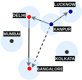
With this argument, we turn our attention towards a different class of problems called all-pairs approximate shortest path problems. As suggested above, these solutions give an approximation of the shortest path between any pair of vertices. One of the inspirations behind this solution is real-life air/road travel (mentioned in Prof. Baswana's slides):
To understand this even better, visualize this problem from the perspective of triangle inequality:
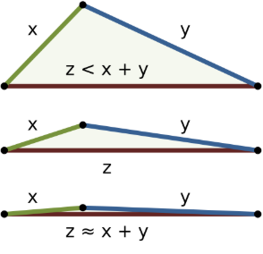
Image by WhiteTimberwolf and licensed under Creative Commons Attribution-Share Alike 3.0 Unported.
From each vertex, if we store distance information to a small number of vertices, can we still be able to report distance between any pair of vertices?The above example showed that having distance information on nearby vertices which in turn have distance information of many other vertices is certainly a useful feature. The above blockquote is from Chapter 39 (Randomized Graph Data-Structures for Approximate Shortest Paths) in Handbook of Data Structures and Applications, 2nd Edition.
So what did Thorup and Zwick show in their paper on Approximate Distance Oracles? And why is it important? From the same chapter:
Among all the data-structures and algorithms designed for computing all-pairs approximate shortest paths, the approximate distance oracles are unique in the sense that they achieves simultaneous improvement in running time (sub-cubic) as well as space (sub-quadratic), and still answers any approximate distance query in constant time. For any \(k \ge 1\), it takes \(O(kmn^{1/k})\) time to compute (2k − 1)-approximate distance oracle of size \(O(kn^{1+1/k})\) that would answer any (2k − 1)-approximate distance query in O(k) time.
Approximate Distance Oracles
To begin, why does the name contain the word oracle? The literal definition of oracle is "a place at which divine advice or prophecy was sought." From the original paper's abstract:
The most impressive feature of our data structure is its constant query time, hence the name “oracle”.Let us start by intuitively understanding the algorithms of a much simpler version known as the 3-approximate distance oracles. Any approximate distance oracle requires two algorithms - a preprocessing/construction algorithm and a distance query algorithm. The preprocessing algorithm constructs the foundation upon which the distance queries can be answered within a constant time. This is similar to the formulation of the matrix in the Floyd-Warshall algorithm.
Preprocessing algorithm for 3-approximate distance oracles
Assume that the set of vertices we have is labeled as V. For example, in the Ten Blocks city, V = {B1, B2, B3, ..... , B10}. While researching on this topic, the most intuitive preprocessing algorithm I found was that described by Prof. Baswana and Prof. Sen (chapter 39):Before intuitively understanding the algorithm, let's first see it in action. We start by choosing \( \gamma = n^{-1/2} = 1/\sqrt{n} \). We will later understand why this is the optimal value to choose. Step 1 can be implemented in the following manner:
- Let \(R \subset V\) be a subset of vertices formed by picking each vertex randomly independently with probability \( \gamma \) (the value of \( \gamma \) will be fixed later on).
- For each vertex \( u \in V \), store the distances to all the vertices of the sample set R.
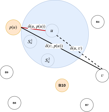
- For each vertex \( u \in V \), let \( p(u) \) be the vertex nearest to \( u \) among all the sampled vertices, and let \( S_{u} \) be the set of all the vertices of the graph G that lie closer to u than the vertex \( p(u) \). Store the vertices of set \( S_{u} \) along with their distance from \( u \).
import random, math
# Based on the Ten Blocks graph
n = 10
V = range(1, n+1)
gamma = 1/math.sqrt(n)

# gamma comes about 0.316
R = [vertex for vertex in V if
    random.choices([True, False], weights=[gamma, 1-gamma])[0]==True]
R as [1, 10].
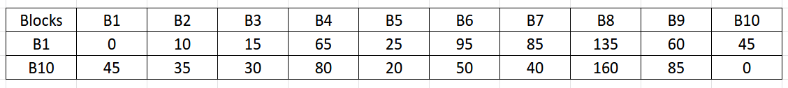
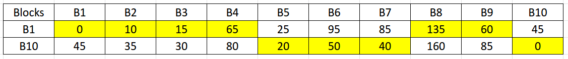
While the above algorithm is ambiguous about the distance metric in step 2, in reality, we want to store the shortest distances from all the vertices in V to those in sample set R. These distances can be calculated using Dijkstra's single-source shortest-path algorithm. However, do note the difference here! We only need to calculate Dijkstra's algorithm with the subset R as our source vertices (i.e. for our case, we need to perform the algorithm twice, one with source vertex as 1 and another with source vertex as 10). Here is the resulting matrix we are to obtain after step 2:
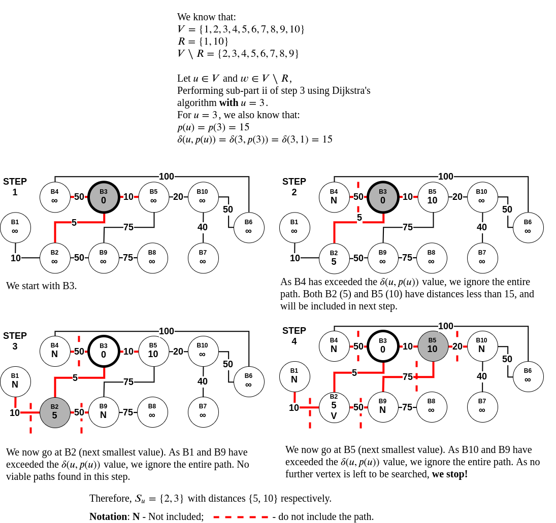
Observing closely, step 3 has two sub-parts. For each \( u \in V \):
- Find \( p(u) \) which is the nearest vertex to \( u \) among all the sampled vertices.
- For each vertex u, find \( S_{u} \) which is the set of all the vertices of the graph G that lie closer to u than the vertex \( p(u) \).
- We only need to calculate the shortest distances between the pairs of each vertex in \( V \) and \( V\setminus R \). This is to avoid any redundant calculations as we have already found the distances between each vertex in V and set R in step 2.
- The symbol \( \setminus \) stands for set-minus and is used in set-theory to find the relative complement of any set A wrt a set B. For example, if A = {1,2,3,4} and B = {3, 5, 7}, then \( A\setminus B \) = {1, 2, 4}. In our case, \( V\setminus R \) = {2, 3, 4, 5, 6, 7, 8, 9}.
- For any pair \( (u, w) \) where \( u \in V \) and \( w \in V\setminus R \), we can stop computing Dijkstra’s algorithm when that pair's distance (let this distance be \( \delta(u, w) \)) exceeds the value \( \delta(u, p(u)) \). That is, when \( \delta(u, w) \ge \delta(u, p(u)) \).
Distance query algorithm for 3-approximate distance oracles
An Analogy
Before we understand the actual algorithm, let us discuss a thought process. Imagine you and your friend wants to meet for a get-together. If either of you knows the other's location, this task becomes simple - you meet at the known person's place. However, if you don't know each other's location and you don't want to bother asking for one, you can meet at a common/famous location, which can act as a middle ground. In the above preprocessing algorithm, \( S_{u} \) (or vertices that lie closer to u than the vertex \( p(u) \)) forms the known location, which is so close that there is no point in meeting at any other common location. However, the vertices in set R act as the common locations, which helps you meet your destination without explicitly looking for it. This means that these common locations do the task of managing all the other locations for vertices in set \( V\setminus R \).
Algorithm
Based on the algorithm described by Prof. Baswana and Prof. Sen (chapter 39):
Let \( u, v \in V \) be any two vertices whose intermediate distance is to be determined approximately.Let us discuss the above blockquote point-wise:
- If either \( u \) or \( v \) belong to set \( R \), we can report exact distance between the two.
- Otherwise also exact distance \( \delta(u,v) \) will be reported if \( v \) lies in \( S_{u} \) or vice versa.
- The only case, that is left, is when neither \( v\in S_{u} \) nor \( u\in S_{v} \). In this case, were report \( \delta(u, p(u)) + \delta(v, p(u)) \) as approximate distance between \( u \) and \( v \). This distance is bounded by \( 3\delta(u, v) \).
- We have stored the exact distance from each vertex \( u \in V \) to all the vertices in set R (see preprocessing algorithm - step 2). We can use this to report the distance in O(1) time.
- If \( v \in S_{u} \) or \( u \in S_{v} \), then this means that either \( u \) or \( v \) or both lie in the other's locality. According to preprocessing algorithm - step 3, we have stored the vertices of set \( S_{u} \) along with their distance from \( u \). We can use this to report the distance in O(1) time.
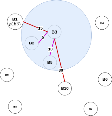
- The last case is inspired by the triangle-inequality example in the all-pairs approximate shortest-path section. When neither \( v\in S_{u} \) nor \( u\in S_{v} \), and \( u \) or \( v \) do not belong to set \( R \), we can use \( p(u) \) to approximate the distance between \( u \) and \( v \). Like the air-travel analogy, wherein Delhi formed as the closest airport to Kanpur to reach Bangalore, in 3-approximate distance oracles, \( p(u) \) plays the role of Delhi. Furthermore, by finding the distance \( \delta(u, p(u)) + \delta(v, p(u)) \), we can use the triangle inequality to approximate the actual distance between \( u,v \) (i.e. \( \delta(u, v) \)).
Therefore, as proved above, for two vertices, the distance reported by 3-approximate distance oracles is no more than three times the shortest distance between these two vertices. Hence the name, 3-approximate distance oracles. However, there are still a few questions left unanswered in this section, like:
- \( \delta(u, p(u)) + \delta(v, p(u)) \le \delta(u, p(u)) + (\delta(v, u) + \delta(u, p(u))) \)
- As by traingle inequality: \( \delta(v, p(u)) \le \delta(v, u) + \delta(u, p(u)) \)
- However, \( \delta(u, p(u)) + (\delta(v, u) + \delta(u, p(u))) = 2\delta(u, p(u)) + \delta(u, v) \)
- As graph is undirected: \( \delta(v, u) = \delta(u, v) \)
- Therefore, \( \delta(u, p(u)) + \delta(v, p(u)) \le 2\delta(u, p(u)) + \delta(u, v) \)
- Finally, \( \delta(u, p(u)) + \delta(v, p(u)) \le 2\delta(u, v) + \delta(u, v) \)
- This is because, \( \delta(u, p(u)) < \delta(u, v) \)
- Hence, \( \delta(u, p(u)) + \delta(v, p(u)) \le 3\delta(u, v) \)
- Why did we choose \( \gamma = n^{-1/2} \) as our probability of a vertex getting picked in set \( R \)?
- How are the distances stored?
(2k-1)-approximate distance oracles
Why \( 2k-1 \)? From Thorup and Zwick:
The approximate distances produced by our algorithms are of a finite stretch. An estimate \( \hat{\delta}(u, v) \) to the distance \( \delta(u, v) \) from \( u \) to \( v \) is said to be of stretch \( t \) if and only if \( \delta(u, v) \le \hat{\delta}(u, v) \le t . \delta(u, v) \). ..... The stretch of the approximations returned is at most \( 2k − 1 \).This means that for generalized approximate distance oracles, \( \delta(u, v) \le \hat{\delta}(u, v) \le (2k-1) . \delta(u, v) \), i.e. \( t = 2k-1 \). Furthermore, when \( k = 1 \), we obtain \( \delta(u, v) \le \hat{\delta}(u, v) \le \delta(u, v) \), which is the classical APSP problem. Moreover, if we insert \( k = 2 \), we obtain the already studied 3-approximate distance oracles. Therefore, for any integer \( k\ge 1 \), \( 2k-1 \) times the actual shortest path is the upper bound for the approximate shortest path calculated using approximate distance oracles. The derivation of the above equation will be explained later in this section.
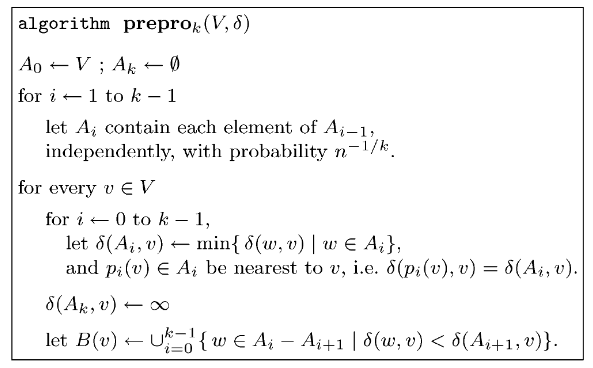
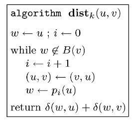
The preprocessing and distance query algorithms for (\(2k-1\))-approximate distance oracles (as presented in Thorup and Zwick):
Dissecting the Preprocessing Algorithm
For our 3-approximate distance oracles, we used a single set \( R \) which was a subset of the set of all vertices in a graph \( V \). For each \( u \in V \), this subset was calculated randomly independently with a probability of \( n^{-1/2} \). The (\(2k-1\))-approximate distance oracles have a similar start. We begin by initializing two subsets:
- \( A_0 \) contains all the vertices present in \( V \).
- \( A_k \) is \( \emptyset \) (an empty set).
import random
def get_subsets(n, k, V):
    """
    n: number of vertices
    k: integer greater than 1 for stretch of (2k-1)
    V: vertices in the graph
    """
    if k < 1:
        raise ValueError("K must be greater than 1 as for " \
            "approximate distance oracles we are dealing with positive edge weights.")

    gamma = n**(-1/k)
    A = dict()
    A[0], A[k] = V, list()

    for i in range(1, k):
        A[i] = [vertex for vertex in A[i-1] if
                    random.choices([True, False], weights=[gamma, 1-gamma])[0]==True]

    return A
In the following, for simplicity, we assume that \( A_{k-1} \ne \emptyset \). This is the case with extremely high probability, and if not, we can just rerun the algorithm.
Let us assume that when the above code is executed on The Ten Blocks graph, with k=3, we get the following output:
>>> get_subsets(10, 3, range(1, 11))
{0: range(1, 11), 3: [], 1: [1, 5, 6, 10], 2: [1, 10]}
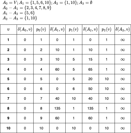
As we will later see in the distance query section(cite this!), for a pair \((u, v)\), we are interested in finding a common vertex (i.e. a vertex which has shortest paths from \( u\) and \(v\)) such that this common vertex is as close to either \(u\) or \(v\) as possible. The above \(p_i(v)\) values help us find that common vertex. And we do, the \(\delta(A_i, v)\) value helps us find the approximate path distance.
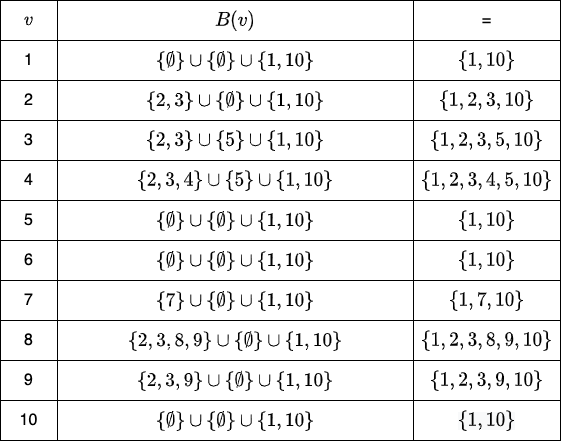
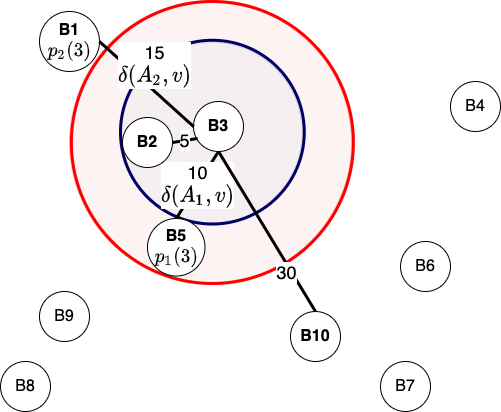
Finally, for every \( v \in V \), we calculate \( B(v) \), which is a set of all vertices, wherein the distance \( \delta(w, v) \) (here \( w \) is formed by applying the relative complement of two sets - \( A_i \setminus A_{i+1} \), i.e. \( w \in A_i \setminus A_{i+1} \)) is less than the distance from all the vertices of \( A_{i+1} \) (i.e. \(\delta(A_{i+1}, v))\). Visualization for the same is:
Dissecting the Distance Query Algorithm
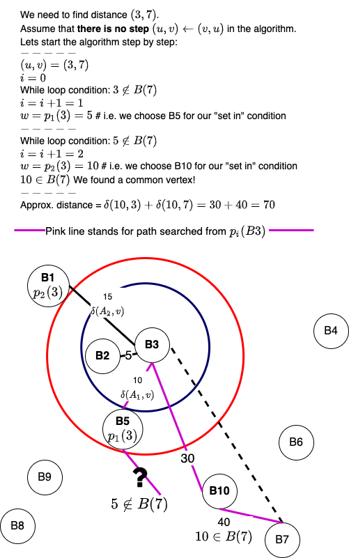
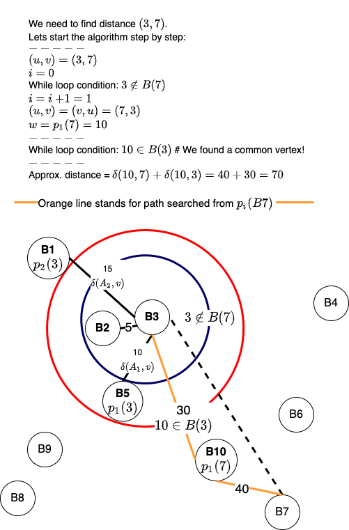
We start the algorithm by initializing \(w = u, i = 0\) and then ask a simple question, is the vertex \(w\) in set \(B(v)\)? We are interested in understanding whether, with the present \(w\), the paths \(\delta(w, u)\) and \(\delta(w, v)\) have been calculated and stored in the pre-processing step. This is similar to finding the common location in 3-approximate distance oracles. However, the difference is that for generalized distance-oracles, we have multiple \(p_i(u)\) instead of one. Notice that in each iteration of the while-loop, we increment \( i\) and calculate \(w = p_i(u)\).
What would happen if we don't execute the line \((u, v) \leftarrow (v, u)\)? Here is a visualization for the same:
Miscellaneous Questions
How are the distances stored?
From the paper by Thorup and Zwick:
The data structure constructed by the preprocessing algorithm stores for each vertex \(v \in V\),For the 2-level hash table, Thorup and Zwick have cited Fredman, Komlós & Szemerédi (1984) who helped develop the perfect hashing scheme for static sets. As mentioned in Introduction to Algorithms (Cormen, et. al.), perfect hashing provides excellent worst-case performance (\(O(1)\) memory access to perform a search, and can limit the space used to \(O(n)\)) when the set of keys is static, which is presently the case for approximate distance oracles. Do note that we have not dealt with dynamic graphs in this blog post. For dynamic graphs, it will be interesting to observe the performance of cuckoo hashing. Coming back to the structure of 2-level hashing, from Introduction to Algorithms (Cormen, et. al.):
- for \(0 \le i \le k−1\), the witness \(p_i(v)\) and the corresponding distance \(\delta(p_i(v), v) = \delta(A_i, v)\).
- the (2-level) hash table for the bunch \(B(v)\), holding \(\delta(v,w)\), for every \(w \in B(v)\).
The first level is essentially the same as for hashing with chaining: we hash the \(n\) keys into \(m\) slots using a hash function \(h\) carefully selected from a family of universal hash functions.How do we use the above tables to answer the distance queries? Again, from Thorup and Zwick:
Instead of making a linked list of the keys hashing to slot \(j\), however, we use a small secondary hash table \(S_j\) with an associated hash function \(h_j\). By choosing the hash functions \(h_j\) carefully, we can guarantee that there are no collisions at the secondary level.
The distance \( \delta(w, u) = \delta(p_i(u), u) \) is read directly from the data structure constructed during the preprocessing stage. The distance \( \delta(w, v) = \delta(v,w) \) is returned by the (2-level) hash table of \( B(v) \) together with the answer to the query \( w \in B(v) \).
Can this be used for distance matrix compression?
From Thorup and Zwick:
An interesting application of the above technique is the following: Given a huge \( n × n\) distance matrix that resides in external memory, or on tape, we can efficiently produce a compressed approximate version of it that could fit in a much smaller, but much faster, internal memory. We assume here that it is possible to pick a not too large integer \( k\) such that the internal memory can accommodate a data structure of size \( O(kn^{1+1/k}) \). A random access to an entry in the original external memory matrix is typically in the order of 10,000 times slower than an internal memory access. Thus, our simple \(O(k)\) time distance query algorithm, working in internal memory, is expected to be significantly faster than a single access to the external memory.
Why choose \(n^{-1/k}\) as our probability?
It turns out that the runtime of \((2k-1)\)-approximate distance oracles is \(O(\gamma^{k-1}n + \frac{k-1}{\gamma}m)\). Here \( \gamma \) is the probability of choosing a vertex in a set. When we calculate the derivative of the above equation wrt \(\gamma\), we get:
- \( \cssId{diff-var-order-mathjax}{\tfrac{\mathrm{d}}{\mathrm{d}\gamma}}\left[{\left(\gamma^{k-1}n+\dfrac{k-1}{\gamma}\right)m}\right] = 0\) - [1]
- \( m\left(\left(k-1\right)n\gamma^{k-2}-\dfrac{k-1}{\gamma^2}\right) = 0\)
- \( \dfrac{\left(k-1\right)m\left(n\gamma^k-1\right)}{\gamma^2} = 0\)
- \( \gamma^k = \dfrac{1}{n} = n^{-1} \)
- \( \gamma = n^{-1/k} \)
- \( \left[{\left((n^{-1/k})^{k-1}n+\dfrac{k-1}{(n^{-1/k})}\right)m}\right] = 0\)
- \( \left[{\left((n^{-1/k})^{-1}(n^{-1/k})^{k}n+\dfrac{k-1}{(n^{-1/k})}\right)m}\right] = 0\)
- \( \left[{\left(n^{1/k}+(k-1)n^{1/k}\right)m}\right] = 0\)
- \( (n^{1/k}(1 + k - 1))m = O(kmn^{1/k}) \)
The total size of the data structure is \( O(kn + \sum_{v\in V} |B(v)|) \). In Section 3.3, we show that the expected size of \( B(v) \), for every \( v \in V\), is at most \( kn^{1/k} \). The total expected size of the data structure is, therefore, \( O(kn^{1+1/k}) \).Unfortunately, I am still trying to figure out all the math (especially the initial equation's origin). A great reference for these derivations can be found in Tyler, Mark, Ivy, and Josh's CS 166 project.
Conclusion
In a future blog post, we will discuss how we can find approximate distances for dynamic graphs, the improvements Patrascu and Roditty made to approximate distance oracles, and how we can obtain improved tree covers and distance labelings using the above data structure.
Keep Exploring!
←