If you like this blog post, do subscribe to my RSS feed

Scrambling Eggs for Spotify with Knuth's Fibonacci Hashing

First Published: 08/12/23

He was very late in returning -- so late, that I knew that the concert could not have detained him all the time. Dinner was on the table before he appeared.
"It was magnificent," he said, as he took his seat. "Do you remember what Darwin says about music? He claims that the power of producing and appreciating it existed among the human race long before the power of speech was arrived at. Perhaps that is why we are so subtly influenced by it. There are vague memories in our souls of those misty centuries when the world was in its childhood."
"That's rather a broad idea," I remarked.
"One's ideas must be as broad as Nature if they are to interpret Nature," he answered.
- A Study in Scarlet, Arthur Conan Doyle

A few weeks back, while browsing Hacker News’ second chance pool, I came across a 2014 blog post from Spotify discussing how to shuffle songs.

Now, at first glance, you might think, “How challenging could it be to shuffle songs in a playlist? Can we not randomly shuffle them out?”

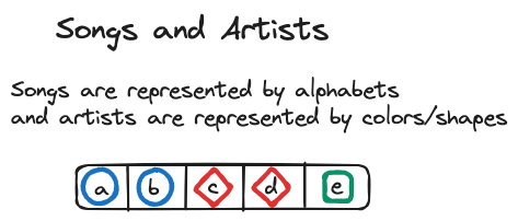
You see, that’s precisely the approach Spotify initially took. They used the Fisher–Yates shuffle to do this. Say you have five songs from three artists, as illustrated in the figure below:

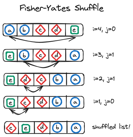
The modern implementation of Fisher–Yates shuffle is an \(O(n)\) time algorithm and can be described as follows:

1. To shuffle an array \(a\) of \(n\) elements (indices \(0..n-1\)):
2. For \(i\) from \(n - 1\) down to \(1\) do
1. \(j \leftarrow \) random integer such that \( 0 \le j \le i \)
2. exchange \(a[j]\) and \(a[i]\)

Using the figure above, we can visualize the algorithm:

Now, this was all fine for the Sweden-based team till they faced a fascinating issue. In their words:

..... We noticed some users complaining about our shuffling algorithm playing a few songs from the same artist right after each other. The users were asking “Why isn’t your shuffling random?”. We responded “Hey! Our shuffling is random!”

At first we didn’t understand what the users were trying to tell us by saying that the shuffling is not random, but then we read the comments more carefully and noticed that some people don’t want the same artist playing two or three times within a short time period.

..... If you just heard a song from a particular artist, that doesn’t mean that the next song will be more likely from a different artist in a perfectly random order. However, the old saying says that the user is always right, so we decided to look into ways of changing our shuffling algorithm so that the users are happier. We learned that they don’t like perfect randomness.

Fascinating indeed! To create an illusion of randomness - randomness with artists evenly spread throughout the playlist - the engineers drew inspiration from a 2007 blog-post by Martin Fiedler.

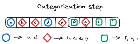
Fiedler’s algorithm is divided into two parts: the merge algorithm and the fill algorithm. Initially, the songs to be shuffled are categorized based on their artist. For instance, assume that we now have three artists and ten songs in our playlist. Then,

The fill algorithm aims to distribute dummy tracks evenly among shorter categories to match the length of the longest one. This step is followed by the merge algorithm, which combines tracks from different categories to form a single playlist in a column-wise fashion.

For example, with the categories mentioned earlier, the fill algorithm would:

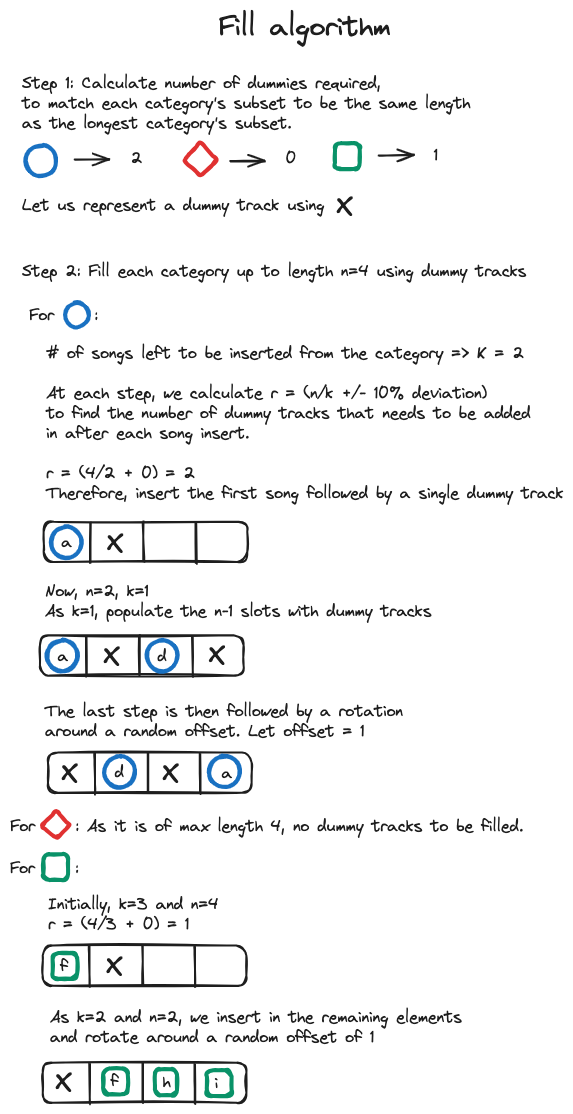
Subsequently, the merge algorithm would create a final playlist as follows:

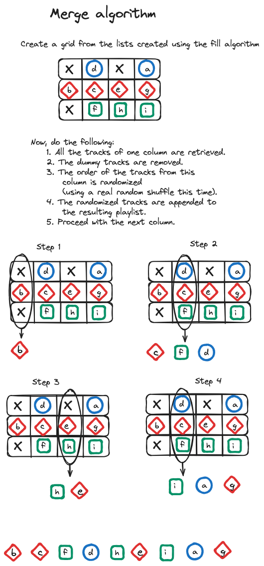
While this method distributes the songs quite efficiently, as mentioned by Spotify, it is complicated and potentially slow in certain scenarios, particularly due to the numerous randomization operations.

Spotify suggested drawing inspiration from existing dithering algorithms, like Floyd–Steinberg dithering, to spread each artist as evenly as possible. Although they don't provide specific details of their algorithm, the basic concept they describe is as follows:

Let’s say we have 4 songs from The White Stripes as in the picture above. This means that they should appear roughly every 25% of the length of the playlist. We spread out the 4 songs along a line, but their distance will vary randomly from about 20% to 30% to make the final order look more random.

We introduce a random offset in the beginning; otherwise all first songs would end up at position 0.

We also shuffle the songs by the same artist among each other. Here we can use Fisher-Yates shuffle or apply the same algorithm recursively, for example we could prevent songs from the same album playing too close to each other.

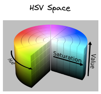
After reading Spotify’s blog post, an idea struck me! You see, a year ago, I wrote a small library to generate aesthetically pleasing colors in the HSV (hue, saturation, value) space.

But how do we define "aesthetically pleasing colors"? And what's the connection to shuffling algorithms?

Let's consider an example where we need to pick five colors to label a chart. Choosing these colors randomly from the RGB space can be quite problematic. Some colors, especially on darker backgrounds, can make text hard to read. Moreover, it is possible to end up with colors that are too similar to each other.

Addressing the issue of dark or light backgrounds turns out to be relatively straightforward – avoid the RGB space and instead, use the HSV space with fixed saturation and value. However, even then, there's a high chance of selecting colors that are too close on the color spectrum. In other words, the selection can be too random, and we might prefer colors that are distributed as evenly as possible across the entire color spectrum.

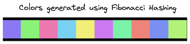
To achieve this, my library employed Fibonacci hashing. The algorithm I implemented was proposed by Martin Leitner‑Ankerl. It utilizes the reciprocal of golden ratio: \[ \Phi^{-1} = \dfrac{\sqrt{5} - 1}{2} \approx 0.618033988749895 \]

As Martin explains in his blog, one of the intriguing properties of the golden ratio is that each subsequent hash value divides the interval into which it falls in accordance with the golden ratio!

To better understand Fibonacci hashing, let us explore it through the perspective of Donald Knuth’s The Art of Computer Programming, Volume 3.

The foundation of Fibonacci hashing is based upon the three-distance theorem. This theorem states: Suppose \(\theta\) is an irrational number. When the points \(\theta\), \((2*theta) % 1\), ….., \((n*theta) % 1\) are placed on a line segment ranging from \(0\) to \(1\) (inclusive), the \(n + 1\) line segments formed will have at most three distinct lengths. Furthermore, the next point \(((n+1)*theta) % 1\) will fall into one of the largest existing segments.

Consider the largest existing segment, spanning from \(a\) to \(c\) (inclusive), being divided into two parts: \(a\) to \(b\) and \(b\) to \(c\). If one of these parts is more than twice the length of the other, we call this division a bad break. Using the three-distance theorem, it can be shown that the two numbers \(\Phi^{-1}\) (the reciprocal of golden ratio!) and \(1 - \Phi^{-1}\) lead to the most uniformly distributed sequences among all numbers \(\theta\) between \(0\) and \(1\). In other words, a break break will occur unless \(\Phi^{-1}\) or \(1 - \Phi^{-1}\) are used.

Using the theory described above, we can now define Fibonacci hashing. However, before diving into that, it is important to first understand multiplicative hashing. Multiplicative hashing involves multiplying a key \(K\) by a constant \(\alpha\). The fractional part of this product is then used to determine the index in a hash table. Fibonacci hashing is a specific variant of multiplicative hashing where the constant \(\alpha\) is set to be the reciprocal of the golden ratio \(\Phi^{-1}\).

And that’s it! We can start at a random hue value between 0 and 1 (this will be our initial key \(K_1\)) and use the Fibonacci hashing from that point to evenly select colors on the color spectrum.

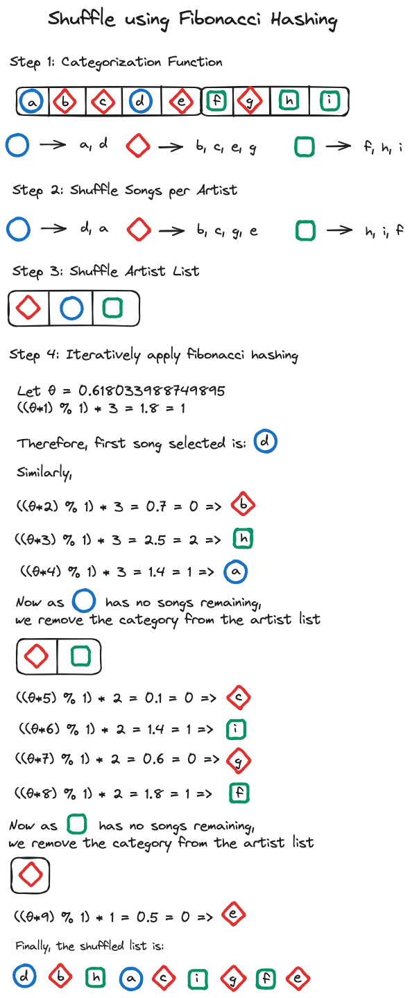
So how can we apply all of this to shuffle songs? Well, the algorithm I came up with is as follows:

1. Categorization Function: Let \(S\) be the set of all songs in the playlist. Define a categorization function \(C: S \rightarrow A\), where \(A\) is the set of artists. This function assigns each song in \(S\) to an artist in \(A\).
2. Shuffle Songs per Artist: For each artist \(a \in A\), shuffle the subset of \(S\) where \(C(s) = A\) for all \(s\) in the subset.
3. Shuffle Artist List: Let \(A’\) be the list of all artists. Apply a random permutation \(\pi\) to \(A’\).
4. Initialize Playlist \(P\): Let \(P\) be an empty list that will store the final shuffled songs.
5. Set Parameters: Initialize \(K=1\) and let \(N = |A|\) (the total number of artists).
6. Select Artist Index: Compute the index \(I = \lfloor ((K * 0.618033988749895) \% 1) * N) \rfloor \).
7. Add Songs to \(P\): Remove the first song from the list of songs corresponding to the artist at \(A’[I]\) and append it to \(P\).
8. Update Parameters: Increment \(K\) by 1.
9. Update Artist List: If the artist at \(A’[I]\) has no remaining songs, decrement \(N\) by 1 and remove the artist from \(A’\).
10. Loop Through: Repeat steps 6 to 9 until \(A’\) is empty. When empty, return \(P\).

If we use a hash table in the categorization function and an array to store the list of all artists, then the overall time complexity of the algorithm would be \(O(S)\).

To compare this algorithm against the naive Fisher-Yates shuffle, I used a measure that calculates the ratio of the count of adjacent song pairs by the same artist to the total number of songs in the playlist minus one. That is,

def measure(shuffled_songs):
    clusters = sum(
        1
        for i in range(len(shuffled_songs) - 1)
        if shuffled_songs[i][‘artist’] == shuffled_songs[i + 1][‘artist’]
    )
    return clusters / (len(shuffled_songs) - 1)    

When the playlist contains songs only from one artist, this measure will be 1. Conversely, when no adjacent song pairs are by the same artist, the measure will return 0.

Using fuzzy testing on a maximum of ten artists, with each having up to ten songs, I generated a million playlists and calculated the statistics for the above algorithm (A) and the fisher-yates shuffle (B). The results were as follows:

• A - Mean: 0.11831, Median: 0.05263, Mode: 0.0, p25: 0.02040, p75: 0.14814, p90: 0.33333, p95: 0.5
• B - Mean: 0.23296, Median: 0.18181, Mode: 0.33333, p25: 0.12121, p75: 0.29629, p90: 0.46666, p95: 0.58333

At first glance, the p95 result might seem surprising. However, this occurs in cases where the fuzzy testing populates a playlist predominantly with songs from a single artist, rendering optimal shuffling infeasible. When a minimum of four songs per artist were used, the results were:

• A - Mean: 0.05948, Median: 0.03703, Mode: 0.0, p25: 0.01694, p75: 0.07843, p90: 0.14285, p95: 0.2
• B - Mean: 0.17223, Median: 0.15555, Mode: 0.2, p25: 0.10909, p75: 0.21875, p90: 0.29268, p95: 0.34482

The results look decent. I’d expect Fiedler’s algorithm to have a near-zero mean, however, the simplicity and speed of the above algorithm does look appealing to me.

And that’s it folks! I hope you enjoyed this little journey. Happy exploring!

Addendum

Recently, I was exploring the “History” section in Knuth’s TAOCP volume 3 to trace back the history of hashing. In it, Knuth states that:

The idea of hashing appears to have been originated by H. P. Luhn, who wrote an internal IBM memorandum in January 1953 that suggested the use of chaining; in fact, his suggestion was one of the first applications of linked linear lists.

Unfortunately, I couldn't locate the memo. It seems they never made it public. However, I stumbled upon a nice paper from 1953 in which he discusses enhancing search engines by refining sets.

Knuth also references Arnold I. Dumey, who appears to be the first to describe hash tables in open literature. I was able to retrieve his paper .

Dumey initiates with an \(O(log\; n)\) solution using the "twenty questions" game, subsequently explaining how we'd be better off if we could do computation before we access the memory. I found his introduction to the hash function rather intriguing:

A certain manufacturing company had a parts and assemblies list of many thousands of items. A mixed digital and alphabetic system of numbering items was used, of six positions in all. Eight complex machines or assemblies were sold to the public. These had item numbers taken from the general system. In setting up a punch card control system on these eight items it was first proposed to record the entire six digit number for each item. However, examination of the eight assembly numbers disclosed that no two were alike on the fourth digit. It was therefore sufficient, for sorting purposes, merely to record the fourth digit, thereby releasing five badly needed information spaces for other purposes.

This rather extreme case indicates that an examination of the item description may disclose a built-in redunancy which can be used to cut the field down to practical size.

He further discusses handling duplicates and introduces chaining:

Adjust the addressing scheme, according to a method which will be described later, to reduce the number of direct addresses, and use the excess locations to store overflows. Put the overflow address at the tail end of stored item information. What the best reduction is varies from case to case. Note that the expectation of the number of accesses to be made goes up when these methods are used. At each access we check by using the complete item description, usually.

And discusses how a somewhat efficient hash address can be constructed by dividing a prime number and using the remainder:

Consider the item description as though it were a number in the scale of 37 or whatever. Or write it as a binary number by using the appropriate punched tape coding. Divide this number by a number slightly less than the number of addressable locations (the writer prefers the nearest prime). Throw away the quotient. Use the remainder as the address, adjusting to base 10, as the case may be.

←