If you like this blog post, do subscribe to my RSS feed

Bao, a learned system for query optimization

First Published: 17/11/23

The more that you read, the more things you will know. The more that you learn, the more places you'll go.
- Dr. Seuss, I Can Read With My Eyes Shut!

So, recently, I have been exploring papers on optimization strategies for databases. In this process, I occasionally encounter fascinating new research happening in this domain. This blog post is about one such topic.

We will be exploring a 2021 paper published in SIGMOD by Marcus et al. which presents a learned system for query optimization named Bao.

What is query optimization?

One of my favorite textbooks for academic-based explorations in DBMS is "Database System Concepts" by Silberschatz et al. Chapter 13 of the book primarily focuses on query optimization. Additionally, Andy Pavlo's lecture notes on query optimization (14 and 15) provide a good overview of this topic.

As mentioned in Silberschatz et al, query optimization is:

The process of selecting the most efficient query-evaluation plan from among the many strategies usually possible for processing a given query, especially if the query is complex.

According to the book, query optimization can be done at both the relational algebra level and on the query processing side. At the relational algebra level, the system tries to find a query expression that is equivalent to the given expression but with improved execution efficiency. Then, on the query processing side, a detailed strategy is composed to choose the specific indices and select the more efficient algorithms for executing an operation.

These optimization strategies can either be heuristic-based or cost-based. Ideally, a SQL query contains common substructures that a DBMS can recognize and optimize. The heuristic-based approach matches parts of a query with these known substructures to assemble a plan and transform the query. For instance, consider a wildcard operator in a SELECT statement (e.g., SELECT * FROM tableA). A potential heuristic might transform such statements to only select the necessary columns based on the rest of the query. Often, this can significantly reduce the amount of data that needs to be retrieved. The best part of a heuristic-based approach is that it usually requires analyzing only the structural metadata of the database, such as schema, indexes, constraints, and not the data itself.

In contrast, a cost-based strategy requires statistical metadata about the underlying data to estimate the cost of executing equivalent query expressions from a given query expression.

This includes examining the table metadata, which contains information about the column names, their data types, and their respective constraints. It also involves looking at relationship data, such as the primary key and foreign key constraints. Additionally, index metadata, including indexed columns and statistics, like the number of rows in a table (also known as cardinality), the number of distinct values in a column, the average length of column values, and the distribution of data, can potentially be considered.

Most relational DBMS, such as PostgreSQL and MySQL, offer statements like EXPLAIN and ANALYZE to find query optimization plans. They are useful for manually optimizing the performance of SQL queries. From PostgreSQL’s documentation on EXPLAIN:

This command displays the execution plan that the PostgreSQL planner generates for the supplied statement. The execution plan shows how the table(s) referenced by the statement will be scanned — by plain sequential scan, index scan, etc. — and if multiple tables are referenced, what join algorithms will be used to bring together the required rows from each input table.

The most critical part of the display is the estimated statement execution cost, which is the planner's guess at how long it will take to run the statement (measured in cost units that are arbitrary, but conventionally mean disk page fetches). Actually two numbers are shown: the start-up cost before the first row can be returned, and the total cost to return all the rows. For most queries the total cost is what matters, but in contexts such as a subquery in EXISTS, the planner will choose the smallest start-up cost instead of the smallest total cost (since the executor will stop after getting one row, anyway).

Similarly, the PostgreSQL documentation on ANALYZE states the following:

The ANALYZE option causes the statement to be actually executed, not only planned. Then actual run time statistics are added to the display, including the total elapsed time expended within each plan node (in milliseconds) and the total number of rows it actually returned. This is useful for seeing whether the planner's estimates are close to reality.

If you enjoy exploring codebases, I encourage you to check out the where.c file in SQLite which is responsible for query optimization. It’s fascinating to see how Bloom filters are used in SQLite to avoid unnecessary data scans. For instance, they are useful when the number of lookup operations exceeds the number of rows in the target table, or to quickly confirm the absence of values in cases where searches are expected to find zero rows. Similarly, SQLite attempts to omit tables from a join that do not affect the result. Conditions are carefully chosen to ensure this. For instance, as aggregate queries (queries with COUNT, SUM, etc.) often rely on all rows from all the tables to compute an aggregate value, omitting tables could lead to incorrect aggregate results. Therefore, only non-aggregate queries are considered for such optimization. Another condition involves analyzing the references of a table. For instance, if a table is only referenced in its own ON or USING clause and nowhere else (like the SELECT, WHERE, GROUPBY, HAVING clauses), then omitting the table should not affect the output of the query. The entire file is filled to the brim with such wonderful optimization gems!

Bao

In the past decade, learned query optimizers have emerged as a modern approach in DBMS, employing machine learning techniques to optimize SQL queries. Their major advantages include adaptability to changing query patterns and the ability to learn complex patterns and relationships in data, that can otherwise be hard to tackle with rule-based systems.

Bao, introduced in a 2021 paper by Marcus et al. is one such learned query optimizer. The term Bao is an abbreviation of “Bandit optimizer”. The word “Bandit” in Bao’s name comes from its use of Contextual Multi-Armed Bandits (CMABs) for query optimization. The paper’s abstract introduces Bao as follows:

Bao takes advantage of the wisdom built into existing query optimizers by providing per-query optimization hints. Bao combines modern tree convolutional neural networks with Thompson sampling, a well-studied reinforcement learning algorithm. As a result, Bao automatically learns from its mistakes and adapts to changes in query workloads, data, and schema.

As mentioned above, what’s rather fascinating about Bao is that it does not replace the database's native optimizer. That is, Bao does not perform its learning from scratch. Instead, it can be integrated into an existing database as an extension (like a PostgreSQL extension) and offers correction to the database's native optimizer, if and when it's needed.

The paper notes that this approach is particularly useful as it allows low integration cost and translates to shorter training times. Additionally, it helps Bao adapt to changes in query workloads, data, and schema, which it does by utilizing the native query optimizer’s cost and cardinality estimates.

We’ve discussed these estimates in the introduction to query optimization, but think of cost estimates as the computational expense (CPU time, disk I/O, etc.) associated with executing a specific query. The cardinality estimate, on the other hand, is the number of rows a query is expected to process or return back. For example, the cardinality of a join operation would be the number of rows expected from the join and the cardinality of a table is the number of rows in that table. To explore the various cost variables that PostgreSQL keeps track of, check out the Planner Cost Constants.

The paper also offers an illustrative example of this symbiotic relationship:

For instance, on a particular query, the PostgreSQL optimizer might under-estimate the cardinality for some joins and wrongly select a loop join when other join algorithms (e.g., merge join, hash join) would be more effective. This occurs in query \(16b\) of the Join Order Benchmark (JOB), and disabling loop-joins for this query yields a \(3x\) performance improvement. Yet, it would be wrong to always disable loop joins. For example, for query \(24b\), disabling loop joins causes the performance to degrade by almost \(50x\), an arguably catastrophic regression.

Now, let us delve deeper into the nuances of Bao and take a closer look at its underlying architecture.

To nudge the search space of native database optimizers, Bao uses query hints. Think of a single query hint as a strategy that maps an incoming query to a specific execution strategy (or a query plan) that the optimizer can use for that query. For example, one hint set might involve disabling loop joins. Disabling loop joins and exploring alternative join strategies can be particularly useful when both tables involved in the join are large, or when the inner table lacks suitable indexes, leading to a full scan of the inner table for each row in the outer table.

A well-defined query hint set can significantly affect the performance of the underlying ML-based predictive model. As I understand it, these hint sets need to be manually chosen. In their experiments, the authors observed the following about the type of hint sets:

Which hint sets matter the most? Of the 48 hint sets used in our experiments, the top 5 hint sets account for 93% of the improvement over the PostgreSQL optimizer: disable nested loop join (35%), disable index scan & merge join (22%), disable nested loop join & merge join & index scan (16%), disable hash join (10%), and disable merge join (10%). Some of these hint sets help in obvious ways: disabling nested loop joins helps when the cardinality estimator underestimates the size of a join, whereas disabling hash joins helps when the cardinality estimator overestimates the size of a join.

One set of query hints could be empty, which would represent the strategy chosen by the native database optimizer.

Bao’s underlying architecture can be divided into three components. It begins when a user submits a query for optimization. Bao then uses the query and \(n\) hint sets to produce \(n\) query plans, one for each hint set.

Each query plan is transformed into a tree, where each node is a feature vector. The way this is achieved is by first binarizing the query plan into a tree structure. This binarization simplifies the operations in the neural network, which we will examine later. Each node, representing a query plan operator (for example, aggregate, merge join, sort, loop join, etc.) is then encoded as a vector. This vector contains:

• One-hot encoding of the query
• Cardinality and cost information
• Optionally, some cache information

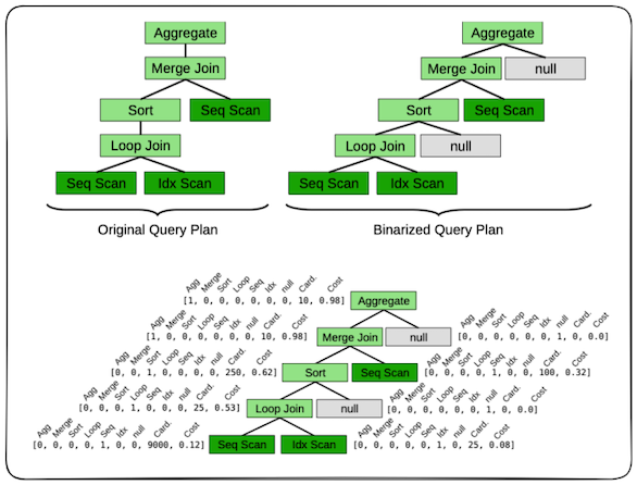
Examples of one-hot encoding and cardinality/cost information of a query are shown in Figure 1. Regarding the cache information representation, the authors state:

Finally, optionally, each vector can be augmented with information from the current state of the disk cache. The current state of the cache can be retrieved from the database buffer pool when a new query arrives. In our experiments, we augment each scan node with the percentage of the targeted file that is cached, although many other schemes can be used. This gives Bao the opportunity to pick plans that are compatible with information in the cache.

To elaborate on the above - in databases, a buffer pool holds frequently accessed data in memory to speed up future read operations. This information is generally fetched when analyzing a query to understand which parts might execute faster. In Bao’s scenario, for each scan node, information about how much of the targeted file is already cached is stored. Think of a scan node as a node that returns raw rows from a table. There can be different methods to retrieve these records, such as sequential scans, index scans, bitmap index scans, etc.

At this point, an interesting question arises: how do we obtain this cache information from, say, PostgreSQL? The paper does not elaborate much on this, however, something like pg_buffercache might be an option. From PostgreSQL’s documentation:

The pg_buffercache module provides a means for examining what's happening in the shared buffer cache in real time.

This module provides the pg_buffercache_pages() function (wrapped in the pg_buffercache view), the pg_buffercache_summary() function, and the pg_buffercache_usage_counts() function.

My assumption is that a query can be written using pg_buffercache to count the number of pages of a table or an index in the buffer cache. Then using relpages from pg_class, we can get the “size of the on-disk representation of this table in pages”. With this data, we can calculate a percentage.

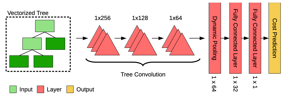
The authors refer to the tree structure described above as a vector tree. This vector tree is fed into a tree convolution neural network (TCNN) that predicts the execution time for each plan. Interestingly, as the query plans are generated independently, this entire process is recommended to be parallelized.

So, what does the TCNN architecture look like? In essence, the architecture (as shown in Figure 2) begins with three layers of tree convolution. This is followed by a dynamic pooling layer and then two fully connected layers, which output the performance prediction.

The motivation behind the initial tree convolution stage is nicely explained in their 2019 paper on Neo (a learned query optimizer that has a similar TCNN architecture):

Tree convolution is a natural fit for Neo. Similar to the convolution transformation for images, tree convolution slides a set of shared filters over each part of the plan tree. Intuitively, these filters can capture a wide variety of local parent-children relations. For example, filters can look for hash joins on top of merge joins, or a join of two relations when a particular predicate is present. The output of these filters provides signals utilized by the final layers of the value network; filter outputs could signify relevant factors such as when the children of a join operator are sorted (suggesting a merge join), or a filter might estimate if the right-side relation of a join will have low cardinality (suggesting that an index may be useful).

The following paragraphs in the Neo paper succinctly describe the convolution stage:

Since each node of the query tree has exactly two child nodes, each filter consists of three weight vectors, \(e_p\), \(e_l\), and \(e_r\). Each filter is applied to each local “triangle” formed by the vector \(x_p\) of a node and two of its left and right child, \(x_l\) and \(x_r\) (0 if the node is a leaf), to produce a new tree node \(x'_p\): \[x'_p = \sigma(e_p \odot x_p + e_l \odot x_l + e_r \odot x_r).\] Here, \(\sigma(·)\) is a non-linear transformation (e.g., ReLU [16]), \(\odot\) is a dot product, and \(x'_p\) is the output of the filter. Each filter thus combines information from the local neighborhood of a tree node. The same filter is “slid” across each tree in an execution plan, allowing a filter to be applied to plans of arbitrary size. A set of filters can be applied to a tree in order to produce another tree with the same structure, but with potentially different sized vectors representing each node. In practice, hundreds of filters are applied. Since the output of a tree convolution is another tree, multiple layers of tree convolution filters can be “stacked.” The first layer of tree convolution filters will access the augmented execution plan tree (i.e., each filter will be slid over each parent/left child/right child triangle of the augmented tree). The amount of information seen by a particular filter is called the filter’s receptive field. The second layer of filters will be applied to the output of the first, and thus each filter in this second layer will see information derived from a node \(n\) in the original augmented tree, \(n\)’s children, and \(n\)’s grandchildren: each tree convolution layer thus has a larger receptive field than the last. As a result, the first tree convolution layer learns simple features (e.g., recognizing a merge join on top of a merge join), whereas the last tree convolution layer learns complex features (e.g., recognizing a left-deep chain of merge joins).

After these layers of tree convolution, a dynamic pooling layer is used to flatten the resulting tree structure into a single vector. Then, two fully connected linear layers map the pooled vector to a single performance prediction. Additionally, ReLU activations and layer normalization are used between these layers. Furthermore, the Adam optimizer is employed during training with a batch size of 16, running until either hundred epochs have elapsed or convergence is reached. The authors define the convergence criteria as a “decrease in training loss of less than 1% over 10 epochs”.

Alright, so we’ve explored the preprocessing stage and the neural architecture. Now it’s time to dig into the heart of this - the training process. How does the training take place? What does the feedback loop look like? A natural decision would be to pick the query plan with the best predicted performance. However, this approach does not work well in practice as the predictions can get skewed towards a few query plans. To address this, the authors suggest a strategy that “balances the exploration of new plans with the exploitation of plans known to be fast”. Such strategies complement reinforcement learning perfectly, leading them to recommend Thompson sampling, a reinforcement learning algorithm, as a learning strategy.

Before understanding Thompson sampling, it is important to motivate the contextual multi-armed bandit problem (CMABs). One of my favorite explanations of the standard multi-armed bandit problem (SMABs) and Thompson sampling is provided by Guilherme Marmerola in his blog post. For a more thorough discourse, I encourage you to explore Chapter 17.3 of Norvig and Russel’s “Artificial Intelligence” book.

From Guilherme’s blog post on SMABs:

The Multi-Armed Bandit problem is the simplest setting of reinforcement learning. Suppose that a gambler faces a row of slot machines (bandits) on a casino. Each one of the \(K\) machines has a probability \(\theta_k\) of providing a reward to the player. Thus, the player has to decide which machines to play, how many times to play each machine and in which order to play them, in order to maximize his long-term cumulative reward.

Thompson sampling is an approximately optimal solution to the multi-armed bandit problem that:

chooses an arm randomly according to the probability that the arm is in fact optimal, given the samples so far.

Bao formalizes its learning strategy in terms of CMABs. Unlike the standard case, CMABs are influenced not only by past rewards but also by additional contextual information available at the time of each decision. In Bao’s case, each arm is a hint set, and the contextual information is the set of query plans produced by the native database optimizer using the query and hint sets. To select the most optimal arm (that is, a hint set), Bao uses Thompson sampling.

The authors formalize it as follows:

Formally, Bao uses a predictive model \(M_\theta\), with model parameters (weights) \(\theta\), which maps query plan trees to estimated performance. This model is used in order to select hint sets for incoming queries. Once a query plan is selected, the plan is executed, and the resulting pair of a query plan tree and the observed performance metric, (\(t_i\), \(P(t_i))\)), is added to Bao’s experience \(E\). Whenever new information is added to \(E\), Bao updates the predictive model \(M_\theta\).

Intuitively, if one wished to maximize exploration, one would choose \(\theta\) entirely at random. If one wished to maximize exploitation, one would choose the modal \(\theta\) (i.e., \(E[P(\theta | E)]\)). Sampling from \(P(\theta | E)\) strikes a balance between these two goals.

The sampling model parameters \(\theta\) from \(P(\theta | E)\) is known as Thompson sampling.

Interestingly, to reduce the training overhead by a factor of \(j\), Bao does not retrain the neural network after every query but instead does so after every \(j^{th}\) query. Moreover, instead of allowing the experience \(E\) to grow unbounded, only the \(k\) most recent experiences are stored.

And that’s an overview of Bao’s architecture. Having observed all of this, let us now explore a broader aspect of Bao. A downside of Bao is that the query optimization time can be substantial, as the native database optimizer needs to run on every query hint to generate query plans. In their experiments, the authors noticed an average overhead of around 200ms. This might not be problematic for long-running queries, but for the ones that are already somewhat performant, using Bao can add significant overhead.

Therefore, Bao is typically suited for workloads that are tail-dominated. Tail latency, simply put, refers to the longer response times experienced by a relatively small percentage of requests in a system. For instance, imagine 80% of the query processing time being spent on 20% of the queries. In their experiments, the authors note that:

In fact, Bao hardly improves the median query performance at all (\(\lt 5\%\)). Thus, in a workload comprised entirely of such "median" queries, performance gains from Bao could be significantly lower.

From what I can gather after reading their experiments section, Bao seems quite performant on tail-dominated workloads. It would be fascinating to compare Bao against some more real-world workloads.

Conclusion

And that’s it, folks! I hope you enjoyed this deep dive into Bao. There are some exciting ideas presented in this paper, and I can’t wait to explore some of the recent works built on top of this. As always, I fully encourage you to explore the paper on your own. There are some fascinating points mentioned on PostgreSQL integration (especially the part on off-policy reinforcement learning), their hardware clusters, and a discussion on Bao’s practicality. Additionally, Ryan Marcus has given a neat talk on this paper that is worth checking out.

←